
This blog explains how large language models (LLMs) are trained and fine-tuned to create systems such as Chat-GPT. We discuss pre-training of models, few-shot learning, supervised fine-tuning, reinforcement learning from human feedback (RLHF), and direct preference optimization. Our previous blog introduced many of these ideas at a high level. In this article, we strive to make these concepts mathematically precise and also to provide insight into why particular techniques are used.
Large language models
For the purposes of this blog, we’ll assume that a large language model refers to a transformer decoder network. The goal of a decoder network is to predict the next word in a partially complete input string. More precisely, this input string is divided into tokens, each of which represents a word or a partial word. Each token is mapped to a corresponding fixed-length embedding. The sequence of embeddings that represent the sentence is fed into the decoder model, which predicts a probability distribution over possible next tokens in the sequence (Figure 1). The next token can be chosen by sampling randomly from this distribution, and then the extended sequence is fed back into the model. In this way, the string is gradually extended. This process is known as decoding. See our previous blogs for other decoding approaches.

Figure 1. Language model overview. A partial input sentence is divided into tokens that represent a word or partial word, and each is mapped to a fixed-length word embedding. These embeddings are passed into the language model, which predicts a probability distribution over the possible next tokens. We choose the next token according to this distribution (here “blue”), and append it to the sentence. By repeating this procedure, the language model can continue the input text in a plausible manner.
Decoder networks comprise a series of transformer layers (Figure 2). Each layer (Figure 3) mixes together information from the token embeddings (using a self-attention mechanism) and processes these embeddings independently (using parallel fully-connected networks). As the embeddings pass through the network, they gradually incorporate more information about the meaning of the whole sequence. The output embedding of the last token in the partial sequence is mapped via a linear transformation and softmax function to a probability distribution over possible values of the subsequent token. Further information about transformer layers and self-attention can be found in our previous series of blogs.

Figure 2. Decoder language model internals. The language model (blue box in Figure 1) of a series of transformer layers. Each receives a set of word embeddings and outputs a set of processed word embeddings. At the final layer, the last embedding is mapped via a linear transformation and softmax function to a probability distribution over possible next tokens.

Figure 3. Each individual transformer layer (gray box in Figure 2) consists of a self-attention layer (in which the embeddings interact with one another) and a set of parallel fully connected networks (in which the embeddings a processed individually). In practice, other components, such as residual connections and layer normalization, are also included to make the model easier to train (not shown).
Pretraining
A vanilla decoder language model has the advantage that it does not require labeled training data. Since the model simply predicts the next token in a sequence, all we need is a large corpus of unlabeled data. We can train the model with partial sequences drawn randomly from this corpus and use the ground truth next token as the label. For simplicity, consider dividing the training data into $I$ sequences $\mathbf{x}_{i}=[x_{i,1},x_{i,2},\ldots,x_{i,T}]$, each containing $T$ tokens. For a model with parameters $\boldsymbol\phi$, the loss function is the sum of the negative log probabilities of the next token $x_{i,t+1}$ given the previous tokens $x_{i,1\ldots t}$ in the sequence :
\begin{equation}
L[\boldsymbol\phi] = -\sum_{i=1}^{I}\sum_{t=1}^{T}\log\Bigl[ Pr(x_{i, t+1}|x_{i, 1 \ldots t},\boldsymbol\phi) \Bigr].
\tag{1}
\end{equation}
In other words, every partial sequence is run separately through the model and adds a single term to the loss function.
However, as the name suggests, large language models are large. At the time of writing, these models typically contain hundreds of billions of parameters and are trained with corpora containing hundreds of billions of tokens (see Table 1 of Zhao et al., 2023). The method described above for training is not very efficient; we must pass $t$ tokens through the model to get just one term for the loss function. Moreover, the partial sequence length $t$ may be significant; the largest systems can consider up to a billion previous tokens.
Masked self-attention
To make training more efficient, the model is modified so that every output embedding (i.e., not just the last embedding) predicts the subsequent token (Figure 4). The first input token becomes a special $\textcolor[rgb]{0.45, 0.30, 0.98}{<start>}$ token, and the first output must predict the first word. The second input is the first word, and the second output must predict the second word, and so on. After training, when we generate new text with the model, we use only the final output to predict the next word.

Figure 4. Efficient training. To improve the efficiency of training, each output predicts a probability distribution over the subsequent token, where the target is the ground truth next word. Here, the first input is the special $\textcolor[rgb]{0.45, 0.30, 0.98}{<start>}$ token and the first output aims to maximize the probability of the first token $\textcolor[rgb]{0.45, 0.30, 0.98}{The}$. The second input is $\textcolor[rgb]{0.45, 0.30, 0.98}{The}$ and the second output must predict the next word $\textcolor[rgb]{0.45, 0.30, 0.98}{fish}$ and so on.
This scheme has the advantage of yielding $t$ loss terms from every sequence of length $t$ that is passed through the model during training. However, if implemented naïvely, the model will have access to the answers during training and can “cheat” by passing these through without learning anything. To prevent the model cheating, the self-attention layer is modified so that each output embedding only receives inputs from the current and previous tokens. This is known as masked self-attention (Figure 5) and prevents the model from “looking ahead” at any stage to find the answer. Whether this pruning of connections has a significant impact on performance is an open question since training by the naïve method would take an impractically long time.
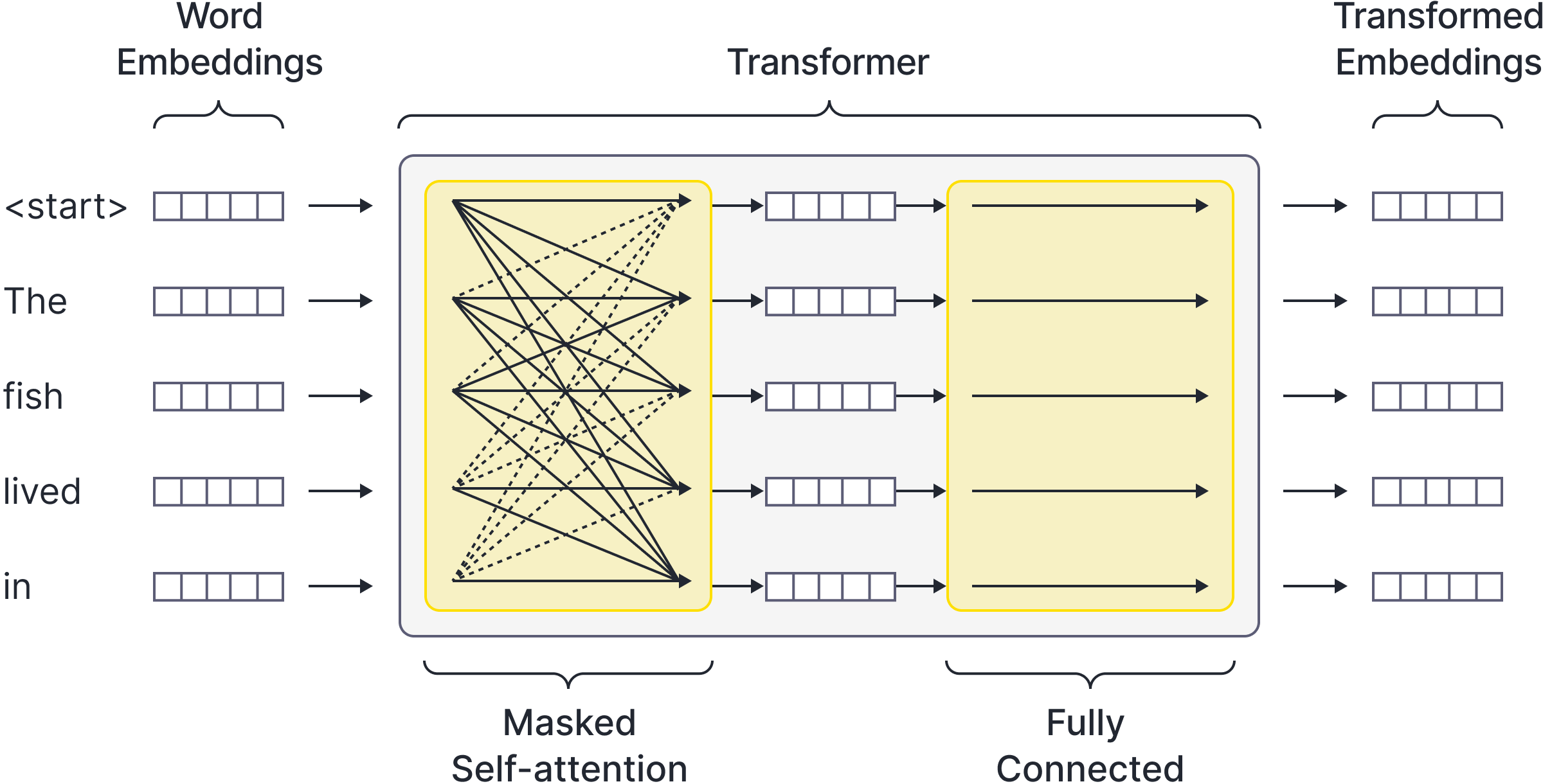
Figure 5. Masked self-attention. To prevent the model cheating by looking ahead in the sequence to find the answer, all upward connections in the self-attention layer (dashed lines) are removed. This means that each output only has access to its corresponding input and those that precede it.
Is this model useful?
What does the model learn from this type of training? It learns the syntax of the language, so it knows that an adjective like cold rarely precedes a verb like jumps. It also learns a lot of common sense knowledge. For example, it can learn that moon is a likely completion of the sentence The astronauts landed on the…. In some limited sense, it has learned about space travel.
The model has an enormous body of knowledge about the world, but it’s not necessarily in a useful form. If we pass the model a question Who was the first man on the moon?…, then the continuation might be the correct answer: …Neil Armstrong. However, it might also treat this as one of a list of questions and continue … What is the largest lake in the world? What is the capital of Canada?. Alternatively, it might treat this as part of a story and continue … was the first question on the exam. I knew the answer but I couldn’t bring it to mind and I panicked. Or, it may reproduce misleading information … This is a trick question. The moon landing was staged.
All of these continuations are statistically plausible based on the statistics of the internet training corpus, so the model is not particularly useful as a chatbot in this form. One trick that can help is to provide some examples of the correct type of response. For example, if we ask the model to continue this text:
Q. Who discovered radium?
A. Pierre and Marie Curie.
Q. Who is the president of the United States?
A. Joe Biden.
Q. Who was the first man on the moon?
A. … ,
then the response will likely be correct. This is sometimes termed in-context or few-shot learning. Although this helps provide a sensible response, it is still not a practical interface for interacting with the model.
Consequently, training from large unlabeled internet corpora in this manner is now considered “pre-training.” To make a useful conversational agent, subsequent stages of fine-tuning help align the model with human needs. Askell et al. (2021) defined aligned models as helpful (they should help the user solve their task), honest (they should not fabricate information or mislead the user), and harmless (they shouldn’t cause physical, psychological, or social harm).
Supervised fine-tuning
The obvious way to solve this problem is to directly train the model to produce desirable responses. This is known as supervised fine-tuning or instruction tuning. It requires a dataset of prompts and ground-truth responses. Sometimes, this is done from scratch. For example, Ouyang et al. (2022) collected 13,000 training prompts and paid people to write responses. In other cases, question-answer pairs are formed by taking existing NLP datasets and reformulating them in question-answer form. For example, Wei et al. (2021) compiled 62 publicly available datasets into this form.
Denoting the tokens for the $i^{th}$ prompt by $\mathbf{x}_i=[x_{i,1},x_{i,2},\ldots ]$ and the tokens in the corresponding response by $\mathbf{y}_i=[y_{i,1},y_{i, 2},\ldots y_{i,T_i}]$, the loss function can now be written as:
\begin{equation}
L[\boldsymbol\phi] = -\sum_{i=1}^{I}\sum_{t=1}^{T_i}\log\Bigl[ Pr(y_{i, t+1}|\mathbf{x}_i, y_{i,1\ldots t},\boldsymbol\phi) \Bigr].
\tag{2}
\end{equation}
where once more $\boldsymbol\phi$ represents the model parameters. This is illustrated in Figure 6. Sometimes, all of the parameters of the model are modified. However, it’s also possible to fix the existing parameters and train new layers at the end of the model or introduce new trainable layers within the model (e.g., Houlsby et al., 2019).

Figure 6. Instruction fine-tuning / supervised fine-tuning. The pre-trained model is fine-tuned using pairs of prompts $\mathbf{x}$ and human-written responses $\mathbf{y}$. In this case the prompt is $\textcolor[rgb]{0.45, 0.30, 0.98}{Describe\; a\; poodle\;}$ and the response is $\textcolor[rgb]{0.45, 0.30, 0.98}{A\; poodle\; is\; a\; type\; of\; dog\; that…}$. The model aims to maximize the probability of the response tokens. In this example and optional $\textcolor[rgb]{0.45, 0.30, 0.98}{<start>}$ token denotes the beginning of the response.
Instruction fine-tuning works extremely effectively. However, it has some disadvantages. First and most importantly, collecting this type of data is extremely expensive. Much painstaking work from educated labelers is needed to produce desirable responses for each prompt. Second, there are many cases where the correct response is not well-defined. For example, if the prompt is Tell me a story about a monkey, no single example response can encompass all the possible responses. Third, while it can encourage certain types of responses, there is no way to discourage possible responses, such as those that use discriminatory language or are insufficiently detailed.
Reinforcement learning from human feedback
One way to address these issues is to train a model based on ratings of real model responses. The work required to rate an existing response is considerably less than providing that response manually. In addition, this scheme allows for multiple possible valid responses and can be used to actively discourage responses that are harmful. The reinforcement learning from human feedback or RLHF pipeline is used to train language models by encouraging them to produce highly rated responses.
One possible problem with this scheme is that it is difficult to attach an absolute rating to a given response. However, it’s easy to compare two or more possible responses and rank which is better. Hence, the RLHF pipeline proceeds in two stages. First, it trains a reward model using the ranking of responses. The reward model outputs a single scalar with the goal that the ranking of these scalars is in accordance with the human rankings. Second, the language model is trained using the reward model, which provides an absolute measure of response quality. For reasons that will become clear, this is done with reinforcement learning. The next two sections consider each of these steps in more detail.
Reward model
To train the reward model, we start with a prompt $\mathbf{x}$ and use the pre-trained or supervised fine-tuned model to generate two responses $\mathbf{y}_1$, and $\mathbf{y}_{2}$. The reward model $r=\mbox{r}[\mathbf{x},\mathbf{y},\boldsymbol\theta]$ has parameters $\boldsymbol\theta$ and ingests the prompt/response combination and returns a scalar reward $r$. Since there are two possible responses $\mathbf{y}_1$ and $\mathbf{y}_2$, we run this model twice to get rewards $r_1$ and $r_2$.
For simplicity, we’ll assume that these are always ordered so that the labeler has indicated they prefer response $\mathbf{y}_{1}$ over $\mathbf{y}_{2}$. The Bradley-Terry probability model assigns the probability that the labeler has ranked the first response as better than the second response according to:
\begin{equation}
Pr(y_{1} > y_{2}) = \frac{\exp\bigl[r_{1} \bigr]}{\exp\bigl[r_{1} \bigr]+ \exp\bigl[r_{2} \bigr]} = \frac{\exp\Bigl[\mbox{r}[\mathbf{x},\mathbf{y}_1,\boldsymbol\theta] \Bigr]}{\exp\Bigl[\mbox{r}[\mathbf{x},\mathbf{y}_1,\boldsymbol\theta] \Bigr]+ \exp\Bigl[\mbox{r}[\mathbf{x},\mathbf{y}_2,\boldsymbol\theta] \Bigr]}
\tag{3}
\end{equation}
Similarly to the softmax function, the exponential maps the rewards $r_1,r_2\in[-\infty,\infty]$ to non-negative numbers and the denominator normalizes the value to make a valid probability distribution. We want to maximize this probability so that the model is in accord with the labelers preferences. As usual, we do this by constructing a loss function based on the negative log-likelihood (Figure 7):
\begin{eqnarray}\label{eq:trainlm_bt}
L[\boldsymbol\theta] &=& -\sum_{i} \log\left[\frac{\exp\Bigl[\mbox{r}[\mathbf{x}_i,\mathbf{y}_{i,1},\boldsymbol\theta] \Bigr]}{\exp\Bigl[\mbox{r}[\mathbf{x}_i,\mathbf{y}_{i,1},\boldsymbol\theta] \Bigr]+ \exp\Bigl[\mbox{r}[\mathbf{x}_i,\mathbf{y}_{i,2},\boldsymbol\theta] \Bigr]}\right]\nonumber \\
&=& -\sum_{i} \log\left[ \frac{1}{1 + \exp\Bigl[\mbox{r}[\mathbf{x}_i,\mathbf{y}_{i,2},\boldsymbol\theta] – \mbox{r}[\mathbf{x}_i,\mathbf{y}_{i,1},\boldsymbol\theta] \Bigr]}\right]\nonumber\\
&=& -\sum_{i} \log\left[= \frac{1}{1 + \exp\Bigl[-\Bigl(\mbox{r}[\mathbf{x}_i,\mathbf{y}_{i,1},\boldsymbol\theta] – \mbox{r}[\mathbf{x}_i,\mathbf{y}_{i,2},\boldsymbol\theta]\Bigr) \Bigr]}\right]\nonumber\\
&=& -\sum_{i} \log\biggl[\mbox{sig}\Bigl[\mbox{r}[\mathbf{x}_i,\mathbf{y}_{i,1},\boldsymbol\theta] – \mbox{r}[\mathbf{x}_i,\mathbf{y}_{i,2},\boldsymbol\theta]\Bigr]\biggr],
\tag{4}
\end{eqnarray}
where $\mathbf{x}_{i}$ is the $i^{th}$ prompt and $\mathbf{y}_{i,1}$ and $\mathbf{y}_{i,2}$ are the two responses to this prompt. Between lines one and two, we have divided the top and bottom by $\exp[\mbox{r}[\mathbf{x}_i,\mathbf{y}_{i,1},\boldsymbol\theta]]$. The function $\mbox{sig}[z]=1/(1+\exp[-z])$ is the logistic sigmoid. The parameters can now be straightforwardly optimized using the backpropagation algorithm.

Figure 7. Reward model. Two responses $\mathbf{y}_1$ and $\mathbf{y}_2$ are sampled from the model. For simplicity, these are ordered so that the labeler prefers $\mathbf{y}_1$ over $\mathbf{y}_2$. They are both passed through the reward model $\mbox{r}[\mathbf{x},\mathbf{y},\boldsymbol\theta]$, and they are compared in the Bradley-Terry loss function.
So far, we haven’t discussed the architecture of the reward model $r=\mbox{r}[\mathbf{x},\mathbf{y},\boldsymbol\theta]$. Unsurprisingly, this, too, is based on transformers. In fact, it is common to fine-tune a copy of the pre-trained model by adding a linear layer to the final output (or perhaps to the average of the outputs) that maps to the single scalar reward value.
Multiple comparisons
The discussion above describes the simplest case where there are only two responses to the given prompt. However, it’s usually more efficient to get the labelers to rank $K$ possible responses. These can be used to generate $\binom{K}{2}$ pairs of responses which can individually contribute to the loss function. Alternatively, we could use the Plackett-Luce probability model, which objects has~$K$ non-negative parameters $\lambda_{1},\lambda_{2},\ldots \lambda_{K}$ and which generalizes the Bradley-Terry to ranking $K$ rewards. It assigns a probability to the labelers ranking, given the underlying rewards $r_{1}\ldots r_{k}$ produced by the model.
Using the reward model
We now have our main model, which can generate a response given any prompt (by sampling the response tokens sequentially and feeding the extended sequence back into the model). We also have a reward model that assigns a scalar value identifying how good that response is. We wish to modify the parameters $\boldsymbol\phi$ of the main model so that it produces responses that are scored highly on average by the reward model.
Ideally, we would train this model by computing the derivatives of a loss with respect to the parameters $\boldsymbol\phi$, where we organize this loss so that it is small when the rewards are high; we would alternate between (i) calculating how a small change in each parameter affects the loss (i.e., compute the derivatives) for the training batch, and (ii) then adjusting the parameters so that the loss decreases. The derivatives are typically computed by working backward through the computation graph using the backpropagation algorithm.
However, this method cannot be used here because we have a stochastic computation graph; the response tokens $y_1,y_2,\ldots$ are sampled randomly one at a time, based on the discrete probability distribution over tokens implied by the main decoder model. The loss function is hence based on the expected value over this sampling step:
\begin{equation}\label{eq:trainlm_rlhf_objective}
L[\boldsymbol\phi] = -\sum_{i=1}^{I}\mathbb{E}_{\mathbf{y}_i|\mathbf{x}_i,\boldsymbol\phi} \Bigl[\mbox{r}[\mathbf{x}_i,\mathbf{y}_i,\boldsymbol\theta] \Bigr],
\tag{5}
\end{equation}
where the distribution $Pr(\mathbf{y}_i|\mathbf{x}_i,\boldsymbol\phi)$ comes from the autoregressive formulation:
\begin{eqnarray}
Pr(\mathbf{y}_i|\mathbf{x}_i,\boldsymbol\phi) = Pr(y_1|\mathbf{x}_i,\boldsymbol\phi)\prod_{t=2}^{T}Pr(y_t|\mathbf{x}_i,y_{i,1:t-1},\boldsymbol\phi).
\tag{6}
\end{eqnarray}
In principle, we could approximate this expectation by drawing sample responses from $Pr(\mathbf{y}_i|\mathbf{x}_i,\boldsymbol\phi)$ and computing the average reward that these samples receive. However, there is no straightforward way to pass the derivatives back through this stochastic graph (Figure 8) and compute:
\begin{equation}
\frac{\partial}{\partial \boldsymbol\phi} \mathbb{E}_{\mathbf{y}_i|\mathbf{x}_i,\boldsymbol\phi} \Bigl[\mbox{r}[\mathbf{x}_i,\mathbf{y}_i,\boldsymbol\theta] \Bigr].
\tag{7}
\end{equation}

Figure 8. Reinforcement learning from human feedback. A prompt $\mathbf{x}$ is fed into the language model $Pr(\mathbf{y}|\mathbf{x},\boldsymbol\phi)$, from which a response $\mathbf{y}$ is sampled token-by-token. The prompt and response are passed to the reward model, which computes the reward. We would like to change the model parameters $\boldsymbol\phi$ so that the rewards are larger on average over the whole batch. To do this, we would need to compute derivatives that calculate how the reward changes when we modify the parameters $\boldsymbol\phi$ using the backpropagation algorithm. However, it is not possible to backpropagate through the sampling step. This motivates the use of reinforcement learning.
To make progress, we perform some algebraic manipulation:
\begin{eqnarray}\label{eq:trainlm_reinforce}
\frac{\partial}{\partial \boldsymbol\phi} \mathbb{E}_{\mathbf{y}_i|\mathbf{x}_i,\boldsymbol\phi}\bigl[\mbox{r}[\mathbf{x}_i,\mathbf{y}_i,\boldsymbol\theta]\bigr] &=& \frac{\partial}{\partial \boldsymbol\phi} \sum_{\mathbf{y}_i} Pr(\mathbf{y}_i|\mathbf{x}_i,\boldsymbol\phi)\cdot \mbox{r}[\mathbf{x}_i,\mathbf{y}_i,\boldsymbol\theta] \nonumber\\
&=& \sum_{\mathbf{y}_i} \mbox{r}[\mathbf{x}_i,\mathbf{y}_i,\boldsymbol\theta] \cdot \frac{\partial}{\partial \boldsymbol\phi}Pr(\mathbf{y}_i|\mathbf{x}_i,\boldsymbol\phi) \nonumber\\
&=& \sum_{\mathbf{y}_i} \mbox{r}[\mathbf{x}_i,\mathbf{y}_i,\boldsymbol\theta] \cdot Pr(\mathbf{y}_i|\mathbf{x}_i,\boldsymbol\phi) \frac{\partial}{\partial \boldsymbol\phi}\log\Bigl[Pr(\mathbf{y}_i|\mathbf{x}_i,\boldsymbol\phi) \Bigr] \nonumber\\
&=&\mathbb{E}_{\mathbf{y}_i|\mathbf{x}_i,\boldsymbol\phi}\left[\mbox{r}[\mathbf{x}_i,\mathbf{y}_i,\boldsymbol\theta] \frac{\partial}{\partial \boldsymbol\phi} \log\Bigl[ Pr(\mathbf{y}_i|\mathbf{x}_i,\boldsymbol\phi)]\Bigr]\right]
\tag{8}
\end{eqnarray}
where we have used the relation $\frac{\partial}{\partial z} \log[\mbox{g}[z]] = (1/\mbox{g}[z]) \frac{\partial}{\partial z}\mbox{g}[z]$ between lines two and three.
This expectation can now be approximated by drawing sample responses $\mathbf{y}_{i}$ from the model and computing the terms straightforwardly. In practice, we might only draw one sample for a very approximate estimate. The derivative now operates on a quantity that precedes the sampling step and can be computed with the backpropagation algorithm.
The result from equation 8 is known as the score function estimator. In the context of reinforcement learning, it is the basis of the REINFORCE algorithm. Indeed, we can think of the main model as an agent that takes sequential actions (choose tokens) and receives a delayed reward from the reward model when the last token is chosen.
Practical matters
In practice, several modifications are commonly made to ensure that this model trains stably.
- The rewards are offset, so the average reward is zero. This reduces the variance of the gradient estimates.
- The loss function in equation 5 is modified to add a second term:
\begin{eqnarray}
\newcommand{\argmin}{\mathop{\rm argmin}}
\newcommand{\argmax}{\mathop{\rm argmax}}
\hat{\boldsymbol\phi}&=& \argmin_{\boldsymbol\phi}\left[-\sum_{i=1}^{I}\mathbb{E}_{\mathbf{y}_i|\mathbf{x}_i,\boldsymbol\phi} \biggl[\mbox{r}[\mathbf{x}_i,\mathbf{y}_i,\boldsymbol\theta] \biggl]-\beta D_{KL}\Bigl[Pr(\mathbf{y}_i|\mathbf{x}_i,\boldsymbol\phi)||Pr(\mathbf{y}_i|\mathbf{x}_i,\boldsymbol\phi^{0})\Bigr] \right]\nonumber \\
\!\!&\!\!=\!\!&\!\!\argmin_{\boldsymbol\phi}\left[-\sum_{i=1}^{I}\mathbb{E}_{\mathbf{y}_i|\mathbf{x}_i,\boldsymbol\phi} \left[\mbox{r}[\mathbf{x}_i,\mathbf{y}_i,\boldsymbol\theta] -\beta \log\left[\frac{Pr(\mathbf{y}_i|\mathbf{x}_i,\boldsymbol\phi)}{Pr(\mathbf{y}_i|\mathbf{x}_i,\boldsymbol\phi^{0})}\right] \right]\right]
\tag{9}
\end{eqnarray}
which penalizes the model if it diverges too far from the initial parameters $\boldsymbol\phi^{0}$ from the supervised fine-tuning stage. Here $\beta$ is a constant scalar that weights the relative contribution of the two terms. - The loss function is optimized with proximal policy optimization (PPO), which clips the gradients so that the policy never changes too much in a single iteration.
- Another term is added to the loss that is the same as for the pretraining. In other words, it encourages the model to still obey the regularities of the language. This also helps ensure that the fine-tuned model is not over-trained and does not depart too much from the initial parameters.
Chat-GPT is based on the InstructGPT model (Ouyang et al. 2022), which uses all of these tricks. Figure 9 shows the relative performance of all of the models discussed so far in this blog.

Figure 9. Instruct GPT results. The rate human observers judge the performance to be better than the supervised fine-tuned model with 175 billion parameters (far right green point). The original pre-trained model generally produces lower-rated responses than the supervised trained model. Performance is improved by adding several examples to the prompt (few-shot learning). Performance increases again with supervised fine-tuning. This can be improved further using reinforcement learning from human feedback. In all cases, the performance increases with model size. Adapted from Ouyang et al. 2022
Direct Preference Optimization
It’s clear from Figure 9 that RLHF can successfully fine-tune large language models so that they are more aligned with human requirements. However, the two-stage system of training a reward model and then using this together with reinforcement learning to fine-tune the original model is overly complex. In addition, reinforcement learning is notoriously unstable, which is why the modifications described in the last section are required.
Recently, a number of methods, including SliC-HF, Stable alignment, Preference ranking optimization, and Direct preference optimization, have been proposed to simplify and improve this performance. In this blog, we concentrate on direct preference optimization, which starts by manipulating the original criterion:
\begin{eqnarray}
\newcommand{\argmin}{\mathop{\rm argmin}}
\newcommand{\argmax}{\mathop{\rm argmax}}
\hat{\boldsymbol\phi}&=& \argmin_{\boldsymbol\phi}\left[-\sum_{i=1}^{I}\mathbb{E}_{\mathbf{y}_i|\mathbf{x}_i,\boldsymbol\phi} \left[\mbox{r}[\mathbf{x}_i,\mathbf{y}_i] -\beta \log\left[\frac{Pr(\mathbf{y}_i|\mathbf{x}_i,\boldsymbol\phi)}{Pr(\mathbf{y}_i|\mathbf{x}_i,\boldsymbol\phi^{0})}\right] \right]\right]\nonumber \\
\!\!&\!\!=\!\!&\!\! \argmin_{\boldsymbol\phi}\left[\sum_{i=1}^{I}\mathbb{E}_{\mathbf{y}_i|\mathbf{x}_i,\boldsymbol\phi} \left[ \log\left[\frac{Pr(\mathbf{y}_i|\mathbf{x}_i,\boldsymbol\phi)}{Pr(\mathbf{y}_i|\mathbf{x}_i,\boldsymbol\phi^{0})}\right]-\frac{1}{\beta}\mbox{r}[\mathbf{x}_i,\mathbf{y}_i] \right]\right]\nonumber \\
\!\!&\!\!=\!\!&\!\! \argmin_{\boldsymbol\phi}\left[\sum_{i=1}^{I}\mathbb{E}_{\mathbf{y}_i|\mathbf{x}_i,\boldsymbol\phi} \left[ \log\left[\frac{Pr(\mathbf{y}_i|\mathbf{x}_i,\boldsymbol\phi)}{Pr(\mathbf{y}_i|\mathbf{x}_i,\boldsymbol\phi^{0})}\right]-\log\left[\exp\left[\frac{1}{\beta}\mbox{r}[\mathbf{x}_i,\mathbf{y}_i]\right]\right] \right]\right]\nonumber \\
\!\!&\!\!=\!\!&\!\! \argmin_{\boldsymbol\phi}\left[\sum_{i=1}^{I}\mathbb{E}_{\mathbf{y}_i|\mathbf{x}_i,\boldsymbol\phi} \left[ \log\left[\frac{Pr(\mathbf{y}_i|\mathbf{x}_i,\boldsymbol\phi)}{Pr(\mathbf{y}_i|\mathbf{x}_i,\boldsymbol\phi^{0})\exp\left[\frac{1}{\beta}\mbox{r}[\mathbf{x}_i,\mathbf{y}_i]\right]}\right]\right]\right]\nonumber
\end{eqnarray}
Now we note that the denominator of this equation is itself an unnormalized probability distribution with partition function (normalizing factor):
\begin{equation}
Z = \sum_\mathbf{y} Pr(\mathbf{y}_i|\mathbf{x}_i,\boldsymbol\phi^{0})\exp\left[\frac{1}{\beta}\mbox{r}[\mathbf{x}_i,\mathbf{y}_i]\right].
\tag{10}
\end{equation}
We can introduce this normalization into the denominator and add a $-\log[Z]$ term to compensate for this:
\begin{eqnarray}
\newcommand{\argmin}{\mathop{\rm argmin}}
\newcommand{\argmax}{\mathop{\rm argmax}}
\hat{\boldsymbol\phi}&=& \argmin_{\boldsymbol\phi}\left[\sum_{i=1}^{I}\mathbb{E}_{\mathbf{y}_i|\mathbf{x}_i,\boldsymbol\phi} \left[ \log\left[\frac{Pr(\mathbf{y}_i|\mathbf{x}_i,\boldsymbol\phi)}{\frac{1}{Z}Pr(\mathbf{y}_i|\mathbf{x}_i,\boldsymbol\phi^{0})\exp\left[\frac{1}{\beta}\mbox{r}[\mathbf{x}_i,\mathbf{y}_i]\right]}\right]-\log[Z]\right]\right] \nonumber\\
\!\!&\!\!=\!\!&\!\! \argmin_{\boldsymbol\phi}\left[\sum_{i=1}^{I}\mathbb{E}_{\mathbf{y}_i|\mathbf{x}_i,\boldsymbol\phi} \left[ \log\left[\frac{Pr(\mathbf{y}_i|\mathbf{x}_i,\boldsymbol\phi)}{\frac{1}{Z}Pr(\mathbf{y}_i|\mathbf{x}_i,\boldsymbol\phi^{0})\exp\left[\frac{1}{\beta}\mbox{r}[\mathbf{x}_i,\mathbf{y}_i]\right]}\right]\right]\right]\nonumber \\
\!\!&\!\!=\!\!&\!\! \argmin_{\boldsymbol\phi}\left[\sum_{i=1}^{I} D_{KL}\left[Pr(\mathbf{y}_i|\mathbf{x}_i,\boldsymbol\phi)\bigg\vert\bigg\vert\frac{1}{Z}Pr(\mathbf{y}_i|\mathbf{x}_i,\boldsymbol\phi^{0})\exp\left[\frac{1}{\beta}\mbox{r}[\mathbf{x}_i,\mathbf{y}_i]\right]\right]\right]\nonumber \\ \tag{11} \\
\end{eqnarray}
where we have abandoned the $-\log[Z]$ term in line two because it does not depend on the parameters $\boldsymbol\phi$. It’s clear that the minimum will be when:
\begin{equation}
Pr(\mathbf{y}_i|\mathbf{x}_i,\boldsymbol\phi)=\frac{1}{Z}Pr(\mathbf{y}_i|\mathbf{x}_i,\boldsymbol\phi^{0})\exp\left[\frac{1}{\beta}\mbox{r}[\mathbf{x}_i,\mathbf{y}_i]\right].
\tag{12}
\end{equation}
Finally, we re-arrange this in terms of the rewards:
\begin{equation}\label{eq:trainlm_rearrange}
\mbox{r}[\mathbf{x}_i,\mathbf{y}_i] = \beta \log\left[\frac{Pr(\mathbf{y}_i|\mathbf{x}_i,\boldsymbol\phi)}{Pr(\mathbf{y}_i|\mathbf{x}_i,\boldsymbol\phi^{0})}\right]+\beta\log[Z].
\tag{13}
\end{equation}
Recall that the loss function for the Bradley-Terry model (equation 4) for ranking two responses with rewards $\mbox{r}[\mathbf{x}_i,\mathbf{y}_{i,1}]$ and $\mbox{r}[\mathbf{x}_i,\mathbf{y}_i,2]$ where the former is ranked higher than the latter is given by:
\begin{eqnarray}
L[\boldsymbol\phi] = -\sum_{i} \log\biggl[\mbox{sig}\Bigl[\mbox{r}[\mathbf{x}_i,\mathbf{y}_{i,1},\boldsymbol\phi] – \mbox{r}[\mathbf{x}_i,\mathbf{y}_{i,2},\boldsymbol\phi]\Bigr]\biggr].
\tag{14}
\end{eqnarray}
where now make the dependence of these terms on the model parameters $\boldsymbol\phi$ explicit (see equation 13).
Substituting our new expression for the rewards, we get:
\begin{eqnarray}
L[\boldsymbol\phi] = -\sum_{i} \log\biggl[\mbox{sig}\left[ \beta \log\left[\frac{Pr(\mathbf{y}_{i,1}|\mathbf{x}_i,\boldsymbol\phi)}{Pr(\mathbf{y}_{i,1}|\mathbf{x}_i,\boldsymbol\phi^{0})}\right] – \beta \log\left[\frac{Pr(\mathbf{y}_{i,2}|\mathbf{x}_i,\boldsymbol\phi)}{Pr(\mathbf{y}_{i,2}|\mathbf{x}_{i},\boldsymbol\phi^{0})}\right]\right]\biggr]. \nonumber \tag{15} \\
\end{eqnarray}
This is a simple expression that can be minimized straightforwardly using backpropagation (Figure 10). It accomplishes the same end as reinforcement learning from human feedback but bypasses explicit reward estimation and is simpler and easier to train. There is experimental evidence that this more direct approach provides better results in both dialogue and text-summarization tasks than using RHLF.

Figure 10. Direct preference optimization. The main model takes a prompt $\mathbf{x}$ used to generate two responses $\mathbf{y}_1$ and $\mathbf{y}_2$. The rewards for each can be computed in terms of the log ratio of the model probability with the new and old parameters. As usual, they are compared using the Bradley-Terry model in the loss function.
Summary
This blog has discussed training and fine-tuning of large language models. The models are pre-trained using an unlabeled corpus to generate the next token for an input string. By feeding the extended sequence back into the model, we can continue the text and generate a response. Unfortunately, the responses from such a model do not necessarily align well with the needs of the user in a chatbot setting. Few-shot learning provides several example prompt/response pairs as part of the input. This gives better results but is not a practical user interface.
We reviewed three methods that fine-tune the model further so that the responses are more useful. The most direct approach is supervised fine-tuning, in which the model learns from example prompt-response pairs. This works well, but the data is costly to acquire. Reinforcement learning from human feedback learns a reward model based on which of several machine-generated responses are preferable to a user. The reward model is then used to train the main model using techniques from reinforcement learning. Finally, direct preference optimization cuts out the reward model and allows direct training from human preference data by standard backpropagation.
A High-level Overview of Large Language Models
Gain valuable insights into essential topics such as LLM training, prompt engineering, concerns, applications, and more. This guide offers curated reading materials for those seeking a deeper understanding of LLMs.