Normalizing Flows are a relatively new class of probabilistic generative model (PGM). Their ease of training and efficiency of sampling and density evaluation make them particularly attractive. Originally introduced in machine learning as a form of non-linear ICA and for use in constructing more expressive posteriors for VAEs, they were quickly picked up as a general form of density estimator. Since then many new forms of normalizing flows have been introduced and they’ve been applied to a diverse range of applications including images, audio, video, reinforcement learning and more. For a more detailed review of normalizing flows check out our recent review article.

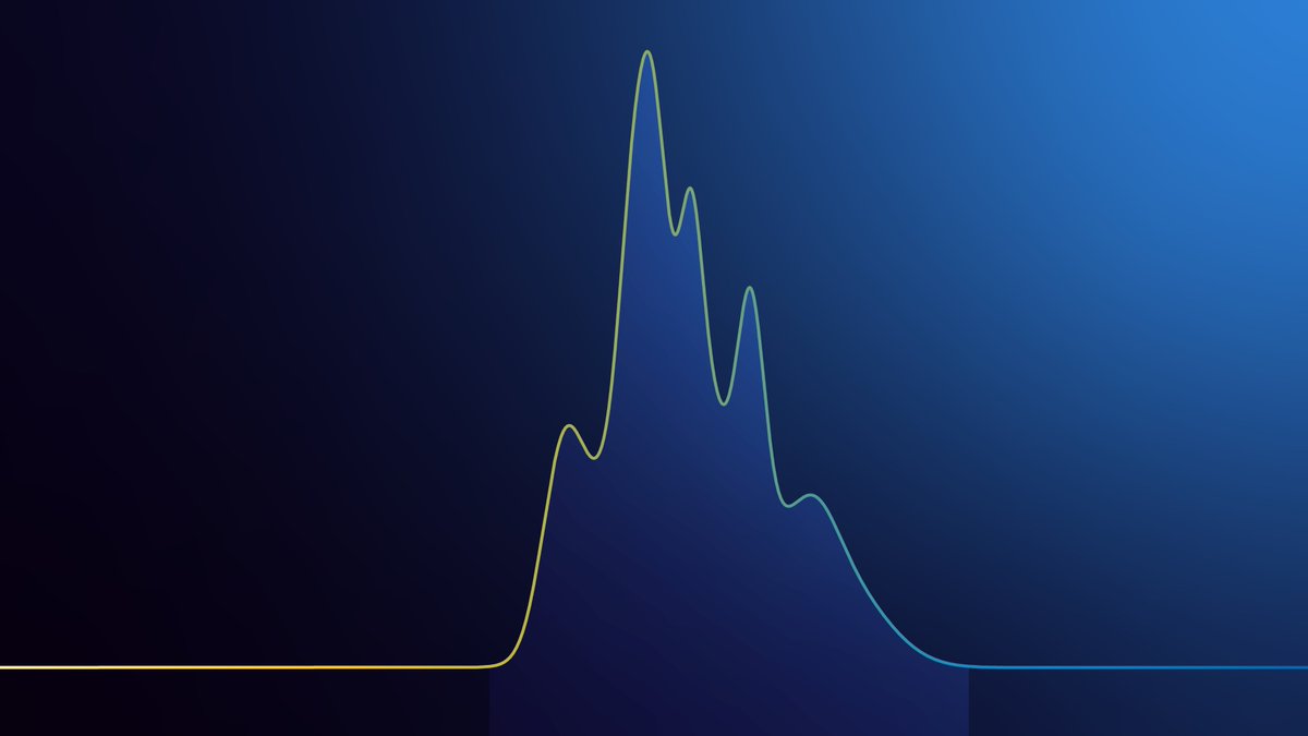
Figure 1. The typical set of a distribution is the region with significant probability, while the tails of a distribution is everything else.
However properties of distributions constructed with normalizing flows remain less well understood theoretically. One important property is that of tail behavior. We can think about a distribution as having two regions: the typical set and the tails which are illustrated in Figure 1. The typical set is what is most often considered; it’s the area where the distribution has a significant amount of density. That is, if you draw samples or have a set of training examples they’re generally from the typical set of the distribution. How accurately a model captures the typical set is important when we want to use distributions to, for instance, generate data which looks similar to the training data. Many papers show figures like Figure 2 which showcase how well a model matches the target distribution in regions where there’s lots of density.

Figure 2. Normalizing Flows are often judged on their ability to approximate the typical set of a distribution. Here different methods are compared by visualizing the density of the typical set. Figure from Sum-of-Squares Polynomial Flows.
The tails of the distribution are basically everything else and, when working on an unbounded domain (like $\mathbb{R}^n$) corresponds to asking how the probability density behaves as you go to infinity. We know that the probability density of a continuous distribution on an unbounded domain goes to zero in the limit, but the rate at which it goes to infinity can vary significantly between different distributions. Intuitively tail behaviour indicates how likely extreme events are and this behaviour can be very important in practice. For instance, in financial modelling applications like risk estimation, return prediction and actuarial modelling, tail behaviour plays a key role.
This blog post discusses the tail behaviour of normalizing flows and presents a theoretical analysis showing that some popular normalizing flow architectures are actually unable to estimate tail behaviour. Experiments show that this is indeed a problem in practice and a remedy is proposed for the case of estimating heavy-tailed distributions. This post will omit the proofs and other formalities and instead will aim at providing a high level overview of the results. For readers interested in the details we refer them to the full paper which was recently presented at ICML 2020.
Normalizing Flows and the Tail Behaviour of Probability Distributions
Let $\mathbf{X} \in \mathbb{R}^D$ be a random variable with a known and tractable probability density function $f_\mathbf{X} : \mathbb{R}^D \to \mathbb{R}$. Let $\mathbf{T}$ be an invertible function and $\mathbf{X} = \mathbf{T}(\mathbf{Y})$. Then using the change of variables formula, one can compute the probability density function of the random variable $\mathbf{Y}$:
\begin{align} f_\mathbf{Y}(\mathbf{y}) & = f_\mathbf{X}(\mathbf{T}(\mathbf{y})) \left| \det \textrm{D}\mathbf{T}(\mathbf{y}) \right| , \tag{1}
\end{align}
where $\textrm{D}\mathbf{T}(\mathbf{y}) = \frac{\partial \mathbf{T}} {\partial \mathbf{y}}$ is the Jacobian of $\mathbf{T}$. Normalizing Flows are constructed by defining invertible, differential functions $\mathbf{T}$ which can be thought of as transforming the complex distribution of data into the simple base distribution, or “normalizing” it. The paper attempts to characterize the tail behaviour of $f_\mathbf{Y}$ in terms of $f_\mathbf{X}$ and properties of the transformation $\mathbf{T}$.
Before we can do that though we need to formally define what we mean by tail behaviour. The basis for characterizing tail behaviour in 1D was provided in a paper by Emanuel Parzen. Parzen argued that tail behaviour could be characterized in terms of the density-quantile function. If $f$ is a probability density and $F : \mathbb{R} \to [0,1]$ is its cumulative density function then the quantile function is the inverse, i.e., $Q = F^{-1}$ where $Q : [0,1] \to \mathbb{R}$. The density-quantile function $fQ : [0,1] \to \mathbb{R}$ is then the composition of the density and the quantile function $fQ(u) = f(Q(u))$ and is well defined for square integrable densities. Parzen suggested that the limiting behaviour of the density-quantile function captured the differences in the tail behaviour of distributions. In particular, for many distributions
\begin{equation} \lim_{u\rightarrow1^-} \frac{fQ(u)}{(1-u)^{\alpha}} \tag{2}\end{equation}
converges for some $\alpha > 0$. In other words, the density-quantile function asymptotically behaves like $(1-u)^{\alpha}$ and we denote this as $fQ(u) \sim (1-u)^{\alpha}$. (Note that here we consider the right tail, i.e., $u \to 1^-$, but we could just as easily consider the left tail, i.e., $u \to 0^+$.) We call the parameter $\alpha$ the tail exponent and Parzen noted that it characterizes how heavy a distribution is with larger values having heavier tails. Values of $\alpha$ between $0$ and $1$ are called light tailed and include things like bounded distributions. A value of $\alpha=1$ corresponds to some well known distributions like the Gaussian or Exponential distributions. Distributions with $\alpha > 1$ are called heavy tailed, e.g., a Cauchy or student-T. More fine-grained characterizations of tail behaviour are possible in some cases but we won’t go into those here.

Figure 3. The density function (top left), cumulative density function (top middle), quantile function (top right) and density-quantile function (bottom left) of a Gaussian and several student T distributions. The density-quantile function $fQ(u)$ is the composition of the density function $f(\mathbf{x})$ with the quantile function $Q(u)$ which is the inverse of the cumulative density function $F(\mathbf{x})$. Plotting $\log 1-u$ vs $\log fQ(u)$ (bottom right) the tail exponent $\alpha$ becomes the slope of the line as $\log 1-u$ goes to $-\infty$ on the left of the figure.
Now, given the above and two 1D random variables, $\mathbf{Y}$ and $\mathbf{X}$ with tail exponents $\alpha_\mathbf{Y}$ and $\alpha_\mathbf{X}$, we can make a statement about the transformation $\mathbf{T}$ that maps between them. First, the transformation is given by $T(\mathbf{x}) = Q_\mathbf{Y}( F_\mathbf{X}( \mathbf{x} ) )$ where $F_\mathbf{X}$ denotes the CDF of $\mathbf{X}$ and $Q_\mathbf{Y}$ denotes the quantile function (i.e., the inverse CDF) of $\mathbf{Y}$. Second, we can then show that the derivative of this transformation is given by
\begin{equation} T'(\mathbf{x}) = \frac{fQ_\mathbf{X}(u)}{fQ_\mathbf{Y}(u)} \tag{3}\end{equation}
where $u=F_\mathbf{X}(\mathbf{y})$ and $fQ_\mathbf{X}$ and $fQ_\mathbf{Y}$ are the density-quantile functions of $\mathbf{X}$ and $\mathbf{Y}$ respectively.
Now, given our characterization of tail behaviour we get that
\begin{equation} T'(\mathbf{x}) \sim \frac{(1-u)^{\alpha_{\mathbf{X}}}}{(1-u)^{\alpha_{\mathbf{Y}}}} = (1-u)^{\alpha_{\mathbf{X}}-\alpha_{\mathbf{Y}}} \tag{4}\end{equation}
and now we come to a key result. If $\alpha_{\mathbf{X}} < \alpha_{\mathbf{Y}}$ then, as $u \to 1$ we get that $T'(\mathbf{x}) \to \infty$. That is, if the tails of the target distribution of $\mathbf{Y}$ are heavier than those of the source distribution $\mathbf{X}$ then the slope of the transformation must be unbounded. Conversely, if the slope of $T(\mathbf{x})$ is bounded (i.e., $T(\mathbf{x})$ is Lipschitz) then the tail exponent of $\mathbf{Y}$ will be the same as $\mathbf{X}$, i.e., $\alpha_\mathbf{Y} = \alpha_\mathbf{X}$.
The above is an elegant characterization of tail behaviour and it’s relationship to the transformations between distributions but it only applies to distributions in 1D. To generalize it to higher dimensional distributions, we consider the tail behaviour of the norm of a random variable, i.e., $\Vert \cdot \Vert$. Then the degree of heaviness of $\mathbf{X}$ can be characterized by the degree of heaviness of the distribution of the norm. Using this characterization we can then prove an analog of the above.
Theorem 3 Let $\mathbf{X}$ be a random variable with density function $f_\mathbf{X}$ that is light-tailed and $\mathbf{Y}$ be a target random variable with density function $f_\mathbf{Y}$ that is heavy-tailed. Let $T$ be such that $\mathbf{Y} = T(\mathbf{X})$, then $T$ cannot be a Lipschitz function.
Tails of Normalizing Flows
So what does this all mean for normalizing flows which are attempting to transform a Gaussian distribution into some complex data distribution? The results show that a Lipschitz transformation of a distribution cannot make it heavier tailed. Unfortunately, many commonly implemented normalizing flows are actually Lipschitz. The transformations used in RealNVP and Glow are known as affine coupling layers and they have the form
\begin{equation} T(\mathbf{x}) = (\mathbf{x}^{(A)},\sigma(\mathbf{x}^{(A)}) \odot \mathbf{x}^{(B)} + \mu(\mathbf{x}^{(A)}) \tag{5}\end{equation}
where $\mathbf{x} = (\mathbf{x}^{(A)},\mathbf{x}^{(B)})$ is a disjoint partitioning of the dimensions, $\odot$ is element-wise multiplication and $\sigma(\cdot)$ and $\mu(\cdot)$ are arbitrary functions. For transformations of this form, we can then prove the following:
Theorem 4 Let $p$ be a light-tailed density and $T(\cdot)$ be a triangular transformation such that $T_j(x_j; ~x_{<j}) = \sigma_{j}\cdot x_j + \mu_j$. If, $\sigma_j(z_{<j})$ is bounded above and $\mu_j(z_{<j})$ is Lipschitz continuous then the distribution resulting from transforming $p$ by $T$ is also light-tailed.
The RealNVP paper uses $\sigma(\cdot) = \exp(NN(\cdot))$ and $\mu(\cdot) = NN(\cdot)$ where $NN(\cdot)$ is a neural network with ReLU activation functions. The translation function $t(\cdot)$ is hence Lipschitz since a neural network with ReLU activation is Lipschitz. However the scale function, $\sigma(\cdot)$, at first glance, is not bounded because the exponential function is not unbounded. However in practice this was implemented as $\sigma(\cdot) = \exp(c\tanh(NN(\cdot)))$ for a scalar $c$. This means that, as originally implemented, $\sigma(\cdot)$ is bounded above, i.e., $\sigma(\cdot) < \exp(c)$. Similarly, Glow uses $\sigma(\cdot) = \mathsf{sigmoid}(NN(\cdot))$ which is also clearly bounded above.
Hence, RealNVP and Glow are unable to unable to represent heavier tailed distributions. Not all architectures have this property though and we point out a few that can actually change tail behaviour, for instance SOS Flows.
To address this limitation with common architectures, we proposed using a parametric base distribution which is capable of representing heavier tails which we called Tail Adaptive Flows (TAF). In particular, we proposed the use of the student-T distribution as a base distribution with learnable degree-of-freedom parameters. With TAF the tail behaviour can be learned in the base distribution while the transformation captures the behaviour of the typical set of the distribution.
Tail Adaptive Flows
We also explored these limitations experimentally. First we created a synthetic dataset using a target distribution with heavy tails. After fitting with a normalizing flow, we can measure it’s tail behaviour. Measuring tail behaviour can be done by estimating the density-quantile function and finding the value of $\alpha$ such that $(1-u)^{\alpha}$ approximates its near $u=1$. Our experimental results confirmed the theory. In particular, fitting a normalizing flow with a RealNVP or Glow style affine coupling layer was fundamentally unable to change the tail exponent, even as more depth was added. Figure 4 shows an attempt to fit a model based on a RealNVP-style affine coupling layers to a heavy tailed distribution (student T). No matter how many blocks of affine coupling layers are used, it is unable to capture the structure of the distribution and the measured tail exponents remain the same as the base distribution.
However, when using a tail adaptive flow the tail behaviour can be readily learned. Figure 5 shows the results of fitting a tail adaptive flow on the same target as above but with 5 blocks. This isn’t entirely surprising as tail adaptive flows use a student T base distribution. However, SOS Flows is also able to learn the tail behaviour as predicted by the theory. This is shown in Figure 6.

Figure 4. Results for RealNVP illustrating its inability to capture heavier tails. The second and third column show the quantile and log-quantile plots for the source, target, and estimated target density. The quantile function of the source and the estimated target density are identical, depicting the inability to capture heavier tails. This is further evidenced by the estimated tail-exponents $\alpha_{\mathsf{source}} = 1.15$, $\alpha_{\mathsf{target}} = 1.81$, and $\alpha_{\mathsf{estimated-target}} = 1.15$.

Figure 5. Quantile and log-Quantile plots for 5 block RealNVP with tail adaptive flows on a student T target. In contrast to the results shown in Figure 4, we are now able to learn the tail behaviour.

Figure 6. Results for SOS-Flows with degree of polynomial $r=2$ for two and three blocks. The first and last column plots the samples from the source (Gaussian) and target (student T) distribution respectively. The two rows from top to bottom in second-fourth columns correspond to results from transformations learned using two, and three compositions (or blocks). The second and third column depict the quantile and log-quantile functions of the source (orange), target (blue), and estimated target (green) and the fourth column plots the samples drawn from the estimated target density. The estimated target quantile function matches exactly with the quantile function of the target distribution illustrating that the higher-order polynomial flows like SOS flows can capture heavier tails of a target. This is further reinforced by their respective tail exponents which were estimated to be $\alpha_{\mathsf{source}} = 1.15$, $\alpha_{\mathsf{target}} = 1.81$, $\alpha_{\mathsf{estimated-target, 2}} = 1.76$, $\alpha_{\mathsf{estimated-target, 3}} = 1.81$.
We also evaluated TAF on a number of other datasets. For instance, Figure 7 shows tail adaptive flows successfully fitting the tails of Neal’s Funnel, an important distribution which has heavier tails and exhibits some challenging geometry.
In terms of log likelihood on a test set, our experiments show that using TAF is effectively equivalent to not using TAF. However, this shouldn’t be too surprising.
We know that normalizing flows are able to capture the distribution around the typical set and this is where most samples, even in the test set, are likely to be. Put another way, capturing tail behaviour is about understanding how frequently rare events happen and by definition it’s unlikely that a test set will have many of these events.

Figure 7. Results for tail-adaptive Real-NVP on Neal’s funnel distribution as target density. The tails became heavier as the number of blocks increased with $\alpha_{\mathsf{source}} = 1.15$, $\alpha_{\mathsf{target}} = 1.63$, and $\alpha_{\mathsf{estimated−target,2}} = 1.36$, $\alpha_{\mathsf{estimated−target,3}} = 1.56$, and $\alpha_{\mathsf{estimated−target,5}} = 1.61$.
Conclusions
This paper explored the behaviour of the tails of commonly used normalizing flows and showed that two of the most popular normalizing flow models are unable to learn tail behaviour that is heavier than that of the base distribution. It also showed that by changing the base distribution we are able to restore the ability of these models to capture tail behaviour. Alternatively, other normalizing flow models like SOS Flows are also able to learn tail behaviour.
So does any of this matter in practice? If the problem you’re working on is sensitive to tail behaviour then absolutely and our work suggests that using an adaptive base distribution with a range of tail behaviour is a simple and effective way to ensure that your flow can capture tail behaviour. If your problem isn’t sensitive to tail behaviour then perhaps less so. However, it is interesting to note that the seemingly minor detail of adding a $\tanh(\cdot)$ or replacing $\exp(\cdot)$ with sigmoid could significantly change the expressiveness of the overall model. These details have typically been motivated by empirically observed training instabilities. However our work connects these details to fundamental properties of the estimated distributions, perhaps suggesting alternative explanations for why they were empirically necessary.