
Introduction
Time-series modeling has in recent years seen vast improvements, owing to the introduction of powerful new deep learning architectures but also to the ever-increasing volume of available training data, in particular in the financial sector. At Borealis AI, we are interested in improving the modeling of real-world time-series data. In capital markets, applications include asset pricing, volatility estimation, market regime classification, and many more. We also consider empirical issues, such as structured dependencies, expressive uncertainty, and non-stationary dynamics. At its core, this quantitative view of market microstructure relies on robust and generalizable representations.
Despite the field’s impressive evolution, dealing with large volumes of data often precludes access to labels and highlights the need for effective self-supervised learning strategies, which have already achieved impressive success in computer vision (e.g., MoCo [1]) and natural language processing(e.g., BERT [2]). While forecasting is inherently self-supervised and therefore can reap some of the benefits of these approaches, namely an ability to utilize unlabelled data, this approach also has some limitations, which motivates the need for alternative self-supervised methods, such as contrastive learning. Three main arguments motivate the use of contrastive approaches:
Firstly, contrastive learning may be more conductive to better generalization. Learning representations through solving a task such as forecasting encourages a model to discard information that is not directly relevant to forecasting. As a consequence, using the same representation for another downstream task might not work as desired. Other fields, such as zero-shot learning, have already noted that contrastive objectives generalize better than other representation learning approaches, including reconstruction and prediction [3]. Contrastive approaches to time-series representation learning have the potential to help solve various challenges in time-series modeling, in particular ones that consider multiple downstream tasks, which is of vital importance for a better understanding of real-world financial data.

Figure 1: Overview of Time-Series Forecasting Methods. The X-axis shows different backbones, the Y- axis different time-series (TS) treatments. Various methods operate at the intersection of backbone model and TS treatments. We show DeepAR [4], Deep State Space [5], ESRNN [6], TS2Vec [7], CoST [8], Autoformer [9], Informer [10], and ScaleFormer [11].
Secondly, contrastive approaches have a higher inherent flexibility than alternatives. As we will see in further sections, contrastive approaches like InfoNCE can be modulated to give more emphasis to strong/weak negative samples, instance or temporal contrast, etc., depending on the needs of the downstream task. Being able to modulate an approach, and having access to a large body of literature on the benefits and drawbacks of different variations, is a significant advantage when it comes to practical applications and can lead to increased robustness with respect to the often challenging properties of financial time-series, such as non-stationarity.
Finally, empirically, contrastive approaches tend to outperform their more traditional counterparts, in particular when large volumes of data are available. In addition to this statement being generally true in the computer vision domain, where contrastive approaches derived from InfoNCE dominate representation learning, similar evidence has also started to emerge for downstream tasks such as time-series classification, forecasting, and anomaly detection, and the field is still quite new!
Background on Time-Series Forecasting
Time-series forecasting plays an important role in many domains, including weather forecasting [12], inventory planning [13], astronomy [14], and economic and financial forecasting [15]. One of the specificities of time-series data is the need to capture seasonal trends [16]. The literature on time-series architectures is vast, and a comprehensive review is beyond the scope of this article; see Fig.1 for a (high-level) overview of the methods discussed below.
Early approaches, such as ARIMA [17] and exponential smoothing [18], were followed by the introduction of neural network-based approaches involving either variants of Recurrent Neural Networks (RNNs)[4,5] or Temporal Convolutional Networks(TCNs) [19]. Time-series Transformers leverage self-attention to learn complex patterns and dynamics from time-series data [20,21]. Binh and Matteson [22] propose a probabilistic, non-auto regressive transformer-based model with the integration of state-space models. The originally quadratic complexity in time and memory was subsequently low ered to O(L log L)by enforcing sparsity in the attention mechanism, e.g., with the ProbSparse attention of the Informer model [10] and the LogSparse attention mechanism [23]. While these attention mechanisms operate on a point-wise basis, Autoformer [9] uses a cross-correlation-based attention mechanism with trend/cycle decomposition, which results in improved performance. ScaleFormer [11] iteratively refines a forecasted time-series at multiple scales with shared weights, architecture adaptations, and a specially-designed normalization scheme, achieving state-of-the-art performance.
Recently, the contrastive learning approach has been applied to time-series forecasting: TS2Vec [7] employs contrastive learning in a hierarchical way over augmented context views to enable a robust contextual representation for each timestamp. CoST [8] performs contrastive learning for learning disentangled seasonal-trend representations for time-series forecasting.
Main Ingredients of Contrastive Learning
General formulation of a contrastive objective
Contrastive learning relies on encouraging the representation of a given example to be close to that of positive pairs while pushing it away from that of negative pairs. The distance used to define the notion of “closeness” is somewhat arbitrary and can commonly be taken to be the cosine similarity. As we will see in the rest of this blog, there is a lot of leeway in terms of defining negative pairs. The InfoNCE loss constitutes the basis of almost all recent methods, in particular in the time-series domain, and variants of it are very commonly used in computer vision and natural language processing. Its standard formulation is:
\begin{align*}
\mathcal{L} = – \sum_{b} \frac{\exp(\mathbf{z}_b \cdot \mathbf{z}^+_b/\tau)}{\exp(\mathbf{z}_b \cdot \mathbf{z}^+_b/\tau) + \sum_{n \in \mathcal{N}_b}\exp(\mathbf{z}_b \cdot \mathbf{z}^-_n / \tau)},
\end{align*}
where $\mathbf{z}^+_b$ is a positive sample(obtained from the example by a set of small random transformations, such as scaling), $\tau$ is a temperature parameter, and the $\mathcal{N}_b$ are negative samples.
The formulation above is very flexible; for instance, one can modify the definition of negative pairs (e.g., to perform contrastive learning in the temporal or instance domain), enhance negative samples to create stronger negatives, adapt the temperature parameter, or change the learning objective itself as exemplified by some of the methods presented in the next section.
Varieties of Contrastive Learning Objectives
In the previous section, we detailed a “standard” learning objective: InfoNCE. A number of alternatives exist to this objective, which we will mention for the sake of completeness. An earlier contrastive loss formulation [24] learns a function that maps an input into a low-dimensional target space such that the norm in the target space approximates the “semantic” distance in the input space. The triplet loss [25] is similar to the modern contrastive loss in the sense that it minimizes the distance between similar distributions and maximizes the distance between dissimilar distributions; however, for the triplet loss, a positive and a negative sample are simultaneously taken as input, together with the anchor sample, to compute the loss. Noise Contrastive Estimation (NCE)[26] uses logistic regression to discriminate the target data from noise.
Most of the more recent contrastive objectives, however, arose as variations of InfoNCE. MoCo [1], which was originally designed for learning image representations but was later applied to time-series, trains a visual representation encoder by matching an encoded query q to a dictionary of encoded keys using a contrastive loss. CoST [8] employs the MoCo variant of contrastive learning to time-series forecasting and makes use of a momentum encoder to obtain representations of the positive pair and a dynamic dictionary with a queue to obtain negative pairs. SimCLR [27] shows that the composition of multiple data augmentation operations is crucial in defining the contrastive prediction tasks that yield effective representations. Additionally, a substantially larger batch can provide more negative pairs. MoCo V2 [28] is an improved version of MoCo replacing its 1-layer fully-connected structure with a 2-layer MLP head with ReLU for the unsupervised training stage. Further modifications include blur augmentation and using a cosine learning rate scheduler.
What constitutes a positive/negative sample?
Contrastive learning approaches rely on defining positive and negative pairs that constitute good priors for the type of information the representation should encode. In the image domain, there are relatively few possibilities to define relevant positive and negative pairs. The most common approach by far holds positive pairs to be augmented versions of an input image, whereas negative pairs are augmented versions of a different image from the dataset. In the time-series domain, however, there are more possibilities.
Instance contrast, where positive pairs are representations from the same example at different time steps and negative pairs are extracted from different examples in a mini-batch, is a natural idea that has been incorporated frequently in recent works. An alternative known as temporal contrast constructs negative pairs from representations of the time-series at distant time steps. Additionally, recent works [8] also consider a contrastive loss in the frequency domain. The different possibilities currently used are listed below and summarized in Figure 2.
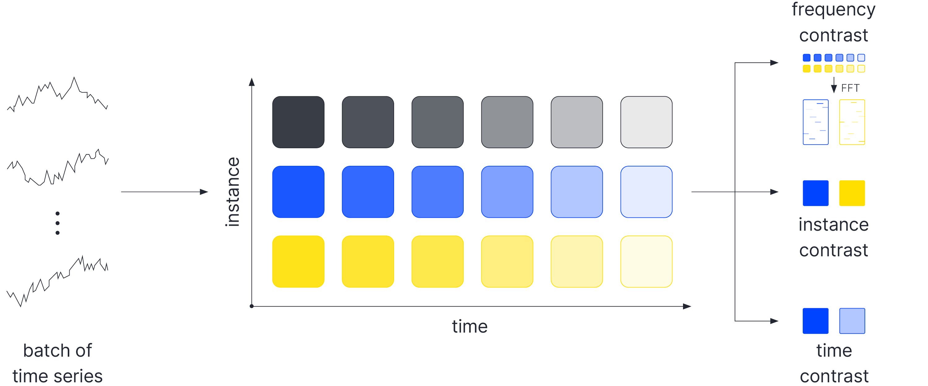
Figure2: Different Approaches to Contrastive Learning for Time-series.
Instance Contrastive Loss. When considering instance contrastive losses, the negative samples are taken from the other examples in the batch. To avoid the constraint imposed by the batch size, methods such as Momentum Contrast(MoCo) maintain a queue of encoded negative samples.
Temporal Contrast. As the time-series encoders yield a representation for each time-step in the original series, another possibility is to draw negative samples from the set of representations of the input example at time steps sufficiently far away. This encourages the representation to maintain high levels of time-specific information.
Contrastive Learning in the Frequency Domain. More recently, analogous losses were introduced in the frequency space by CoST, which first maps the encoded time-series into the frequency domain using an FFT and then computes separate losses by mapping the complex-valued result to its real-valued phase and amplitude. These losses add a strong inductive prior to the learned representation, encouraging it to preserve seasonal information.
Of course, there are many other possibilities, some of which could be the key to learning stronger representations!
Moving Forward
As we have seen, contrastive time-series representation learning has a lot of potential for impactful research, and is a relatively new field. At Borealis AI we care deeply about better understanding real-world time-series, in particular in finance. If you would like to help us improve the performance and robustness of contrastive time-series representation learning we would be happy to hear from you.
References
[1] K. He, H. Fan, Y. Wu, S. Xie, and R. Girshick, “Momentum contrast for unsupervised visual representation learning,” in Proceedings of the IEEE/CVF conference on computer vision and pattern recognition, pp.9729–9738,2020.
[2] J. Devlin, M.-W. Chang, K. Lee, and K. Toutanova, “Bert: Pre-training of deep bidirectional transformers for language understanding,” arXiv preprint arXiv:1810.04805,2018.
[3] T. Sylvain, L. Petrini, and D.Hjelm, “Locality and compositionality in zero-shot learning, “in International Conference on Learning Representations, 2019.
[4] D. Salinas, V. Flunkert, J. Gasthaus, and T. Januschowski, “Deepar: Probabilistic forecasting with autoregressive recurrent networks,” International Journal of Forecasting, vol.36, no.3, pp.1181–1191, 2020.
[5] S. S. Rangapuram, M. W. Seeger, J. Gasthaus, L. Stella, Y. Wang, and T. Januschowski, “Deep state space models for time series forecasting,” Advances in neural information processing systems, vol. 31, 2018.
[6] A. Redd, K. Khin, and A. Marini, “Fast es-rnn: A gpu implementation of the es-rnn algorithm,” arXiv preprint arXiv:1907.03329, 2019.
[7] Z. Yue, Y. Wang, J. Duan, T. Yang, C. Huang, Y. Tong, and B. Xu, “Ts2vec: Towards universal representation of time series,” arXiv preprint arXiv:2106.10466, 2021.
[8] G. Woo, C. Liu, D. Sahoo, A. Kumar, and S. Hoi, “Cost: Contrastive learning of disentangled seasonal trend representations for time series forecasting,” arXiv preprint arXiv:2202.01575, 2022.
[9] J. Xu, J. Wang, M. Long, et al., “Autoformer: Decomposition transformers with auto-correlation for long-term series forecasting,” Advances in Neural Information Processing Systems, vol. 34, 2021.
[10] H. Zhou, S. Zhang, J. Peng, S. Zhang, J. Li, H. Xiong, and W. Zhang, “Informer: Beyond efficient transformer for long sequence time series forecasting, in Proceedings of AAAI, 2021.
[11] A. Shabani, A. Abdi, L. Meng, and T. Sylvain, “Scaleformer: Iterative multi-scale refining transformers for time series forecasting,” arXiv preprint arXiv:2206.04038,2022.
[12] A. H. Murphy, “What is a good forecast? An essay on the nature of goodness in weather forecasting,” Weather and forecasting, vol. 8, no.2, pp. 281–293, 1993.
[13] A. A. Syntetos, J. E. Boylan, and S. M. Disney, “Forecasting for inventory planning: a 50-year review,” Journal of the Operational Research Society, vol. 60, no.1, pp. S149–S160, 2009.
14] J. D. Scargle, “Studies in astronomical time series analysis. i-modeling random processes in the time domain,” The Astrophysical Journal Supplement Series, vol. 45, pp. 1 – 71, 1 981.
[15] B. Krollner, B. J. Vanstone, G. R. Finnie, et al., “Financial time series forecasting with machine learning techniques: a survey.,” in ESANN,2010.
[16] P.J. Brock well and R.A. Davis, Time series: theory and methods. Springer Science & Business Media, 2009.
[17] G.E. Box and G.M. Jenkins, “Some recent advances in forecasting and control, “Journal of the Royal Statistical Society.Series C (Applied Statistics), vol.17, no.2, pp. 91–109, 1968.
[18] R. Hyndman, A.B. Koehler, J.K. Ord, and R.D. Snyder, Forecasting with exponential smoothing: the state space approach. Springer Science & Business Media, 2008.
[19] S. Bai, J.Z. Kolter, and V.Koltun, “An empirical evaluation of generic convolutional and recurrent networks for sequence modeling,” arXiv:1803.01271, 2018.
[20] N. Wu, B. Green, X. Ben, and S.O’ Banion, “Deep transformer models for time series forecasting: The influenza prevalence case,” arXiv preprint arXiv:2001.08317, 2020.
[21] G. Zerveas, S. Jayaraman, D. Patel, A. Bhamidipaty, and C. Eickhoff, “A transformer-based framework for multivariate time series representation learning, “in Proceedings of the 27th ACM SIGKDD Conference on Knowledge Discovery & Data Mining, pp. 2114–2124, 2021.
[22] B. Tang and D.S. Matteson, “Probabilistic transformer for time series analysis,” Advances in Neural Information Processing Systems, vol.34, pp. 23592–23608, 2021.
[23] S. Li, X. Jin, Y. Xuan, X. Zhou, W. Chen, Y. X. Wang, and X. Yan, “Enhancing the locality and breaking memory bottleneck of transformer on time series forecasting,” Advances in Neural Information Processing Systems, vol. 32, pp. 5243 – 5253, 2019.
[24] S. Chopra, R. Hadsell, and Y. LeCun, “Learning a similarity metric discriminatively, with application to face verification,” in 2005 IEEE Computer Science Society Conference on Computer Vision and Pattern Recognition (CVPR’05), vol. 1, pp. 539–546, IEEE, 2005.
[25] F. Schroff, D. Kalenichenko, and J. Philbin, “Facenet: A unified embedding for face recognition and clustering,” in Proceedings of the IEEE conference on computer vision and pattern recognition, pp. 815–823, 2015.
[26] M. Gutmann and A. Hyvärinen, “Noise contrastive estimation: A new estimation principle for unnormalized statistical models, in Proceedings of the thirteenth international conference on artificial intelligence and statistics, pp. 297–304, JMLR Workshop and Conference Proceedings, 2010.
[27] T. Chen, S. Kornblith, M. Norouzi, and G. Hinton, “A simple framework for contrastive learning of visual representations,” arXiv preprint arXiv:2002.05709, 2020.
[28] X. Chen, H. Fan, R. Girshick, and k. He, “Improved baselines and momentum contrastive learning,” arXiv preprint arXIV:2003.04297, 2020.
We're Hiring!
Borealis AI offers a stimulating work environment and the platform to do world-class machine learning in a startup culture. We're growing the team, hiring for roles such as Machine Learning Researcher, Research Director, Product Manager and more.
See all roles