
A knowledge graph (KG) contains a collection of related facts about the world. In practice, the graph will inevitably be incomplete and the task of knowledge graph completion is to infer new facts from the ones that are already known. Sometimes the facts in the graph are associated with a particular timestamp and may or may not be true at other times. In this post, we present a new method for KG completion that takes into account these timestamps. It is based on a new representation that we term diachronic embeddings. The code and datasets for reproducing our results can be found on Github – DE-SimplE.
The structure of this post is as follows. First, we briefly review knowledge graphs and knowledge graph completion in static graphs. Second, we discuss the extension to temporal knowledge graphs. Third, we present our new method for knowledge completion in temporal knowledge graphs and demonstrate the efficacy of this method in a series of experiments. Finally, we draw attention to some possible future directions for work in this area.
Knowledge graphs
Knowledge graphs are knowledge bases of facts where each fact is of the form $(Alice, Likes, Dogs)$. Here $Alice$ and $Dogs$ are called the head and tail entities respectively and $Likes$ is a relation. An example knowledge graph is depicted in figure 1.
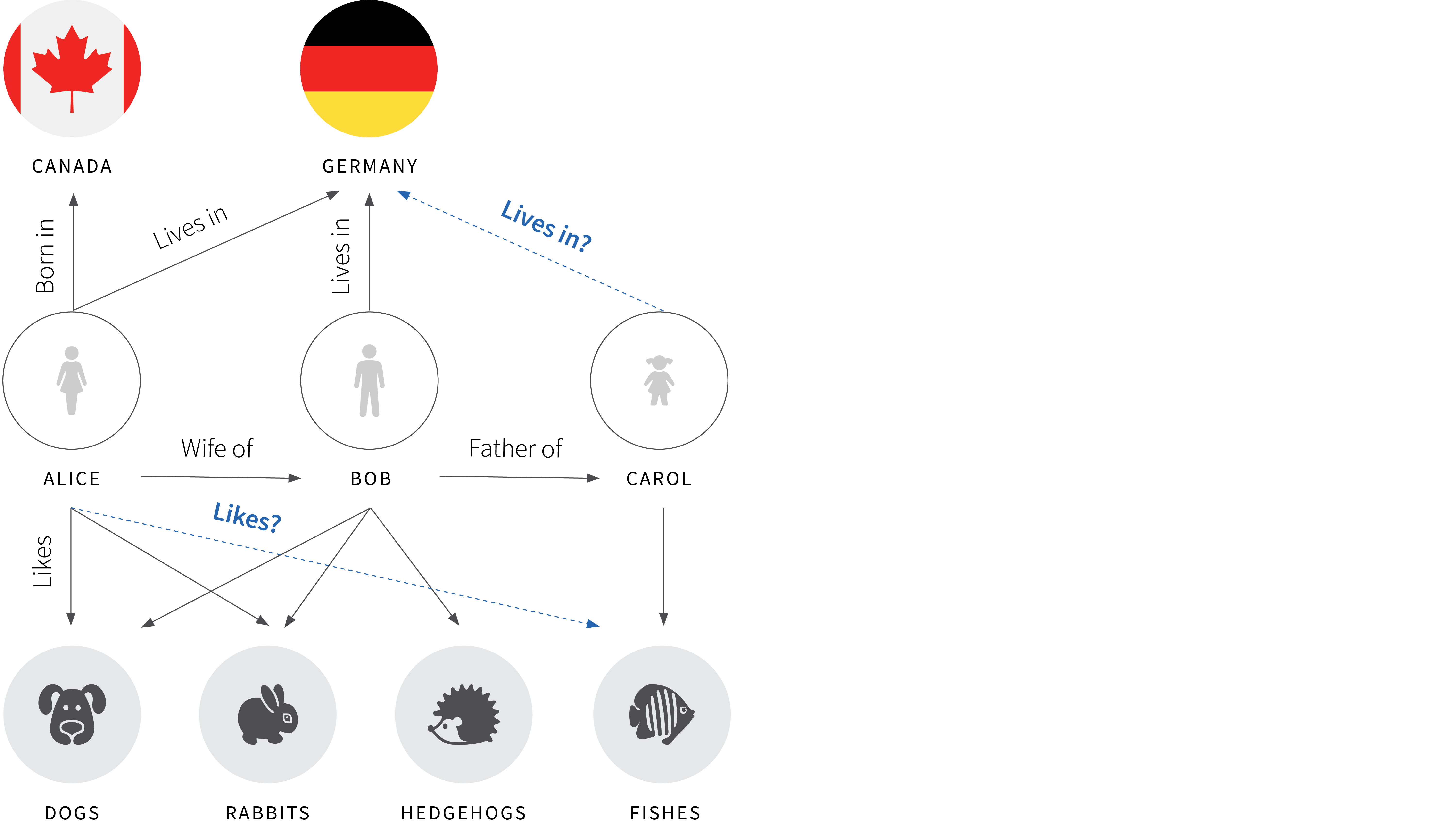
Figure 1. Example knowledge graph. Here, there are three types of entities (countries, people, and animals). Each solid black arrow represents a known relation between the head entity (at the start of the arrow) and the tail entity (at the end). The problem of knowledge graph completion is to infer new facts (dashed blue arrows) based on the existing ones.
KG completion is the problem of inferring new facts from a KG given the existing ones. This may be possible because the new fact is logically implied as in:
\begin{equation*} (Alice, BornIn, London) \land (London, CityIn, England) \implies (Alice, BornIn, England)\end{equation*}
or it may just be based on observed correlations. If $(Alice, Likes, Dogs)$ and $(Alice, Likes, Cats)$ then there’s a high probability that $(Alice, Likes, Rabbits)$.
For a single relation-type, the problem of knowledge graph completion can be visualised in terms of completing a binary matrix. To see this, consider the simpler knowledge graph depicted in figure 2a, where there are only two types of entities and one type of relation. We can define a binary matrix with the head entities in the rows and the tail entities in the columns (figure 2b). Each known positive relation corresponds to an entry of ‘1’ in this matrix. We do not typically know negative relations. However, we can generate putative negative relations, by randomly sampling combinations of head entity, tail entity and relation. This is reasonable for large graphs where almost all combinations are false. This process is known as negative sampling and these negatives correspond to entries of ‘0’ in the matrix. The remainin missing values in the matrix are the relations that we wish to infer in the KG completion process.

Figure 2. a) Simplified knowledge graph. In this graph, there are only two types of entities (people and animals) and a single type of relation $(Likes)$. The solid black lines indicate known positive relations. The solid yellow lines indicate negative relations generated by negative sampling and the dashed blue lines indicate relations that we wish to predict. b) The knowledge completion problem for this graph can be thought of as completing missing values in a binary matrix that encodes the relations between all people and all movies.
Knowledge graph completion as factorization
This matrix representation of the single-relation knowledge graph completion problem suggests a way forward. We can consider factoring the binary matrix $\mathbf{M} = \mathbf{A}^{T}\mathbf{B}$ into the outer product of a portrait matrix $\mathbf{A}^{T}$ in which each row corresponds to the head entity and a landscape matrix $\mathbf{B}$ in which each column corresponds to the tail entity. This is illustrated in figure 3. Now the binary value representing whether a given fact is true or not is approximated by the dot product of the vector (embedding) corresponding to the head entity and the vector corresponding to the tail entity. Hence, the problem of knowledge graph embedding becomes equivalent to learning these embeddings.
More formally, we might define the likelihood of a relation being true as:
\begin{eqnarray}Pr(a_{i}, Likes, b_{j}) &=& \mbox{sig}\left[\mathbf{a}_{i}^{T}\mathbf{b}_{j} \right]\nonumber \\Pr(a_{i}, \lnot Likes, b_{j}) &=& 1-\mbox{sig}\left[\mathbf{a}_{i}^{T}\mathbf{b}_{j} \right] \tag{1}\end{eqnarray}
$\mbox{sig}[\bullet]$ is a sigmoid function. The term $\mathbf{a}_{i}$ is the embedding for the $i^{th}$ head entity (from the $i^{th}$ row of the portrait matrix $\mathbf{A}^{T}$) and $\mathbf{b}_{j}$ is the embedding for the $j^{th}$ tail entity $b$ (from the $j^{th}$ column of the landscape matrix $\mathbf{B}$). We can hence learn the embedding matrices $\mathbf{A}$ and $\mathbf{B}$ by maximizing the log likelihood of all of the known relations.

Figure 3. Knowledge graph completion as factorization. The binary matrix representing the known knowledge relations can be approximated as an outer product of a portrait matrix (where each row contains an embedding for the person) and a landscape matrix (where each column contains an embedding for the animal). These can be learned so that they reconstruct the known data as well as possible and then used to predict the missing relations.
The above discussion considered only the simplified case where there is a single type of relation between entities. However, this general strategy can be extended to the case of multiple relations by considering a three dimensional binary tensor in which the third dimension represents the type of relation (figure 4). During the factorization process, we now also generate a matrix containing embeddings for each type of relation.

Figure 4. Knowledge graph completion for multiple relations can be considered as filling in the missing values in a three-dimensional binary tensor.
Beyond factorization
In the previous section, we considered KG completion in terms of factorizing a matrix or tensor into matrices of embeddings for the head entity, tail entity and relation.
We can generalize this idea, by retaining the notion of embeddings, but use more general score functions than the one implied by factorization to provide scores for each tuple. For example, TransE (Bordes et al. 2013) maps each entity and each relation to a vector of size $d$ and defines the score for a tuple $(Alice, Likes, Fish)$ as:
\[-|| {z}_{Alice} + {z}_{Likes} – {z}_{Fish}||\]
where ${z}_{Alice},{z}_{Likes},{z}_{Fish}\in\mathbb{R}^d$, corresponding to the embeddings for $Alice$, $Likes$, and $Fish$, are vectors with learnable parameters. To train, we define a likelihood such that $-|| {z}_{Alice} + {z}_{Likes} – {z}_{Fish}||$ becomes large if $(Alice, Likes, Fish)$ is in the KG and small if $(Alice, Likes, Fish)$ is likely to be false.
Other models map entities and relations to different spaces and/or use different score functions. For a comprehensive list of existing approaches and their advantages and disadvantages, see Nguyen (2017).
Temporal knowledge graphs
Temporal KGs are KGs where each fact can have a timestamp associated with it. An example of a fact in a temporal KG is $(Alice, Liked, Fish, 1995)$. Temporal KG completion (TKGC) is the problem of inferring new temporal facts from a KG based on the existing ones.
Existing approaches for TKGC usually extend (static) KG embedding models by mapping the timestamps to latent representations and updating the score function to take into account the timestamps as well. As an example, TTransE extends TransE by mapping each entity, relation, and timestamp to a vector in $\mathbb{R}^d$ and defining the score function for a tuple $(Alice, Liked, Fish, 1995)$ as:\[-|| z_{Alice} + z_{Liked} + z_{1995} – z_{Fish}||\]
For a comprehensive list of existing approaches for TKGC and their advantages and disadvantages, see Kazemi et al. (2019).
Diachronic embeddings for temporal knowledge graph completion
We develop models for TKGC based on an intuitive assumption: to provide a score for, $(Alice, Liked, Fish, 1995)$, one needs to know $Alice$’s and $Fish$’s features in $1995$; providing a score based on their current features or an aggregation of their features over time may be misleading. That is because $Alice$’s personality and the sentiment towards $Fish$ may have been quite different in 1995 as compared to now (figure 5). Consequently, learning a static embedding for each entity – as is done by existing approaches – may be sub-optimal as such a representation only captures an aggregation of entity features during time.

Figure 5. In our scheme, entity features may change over time. For example, here Alice's interest in aquatic animals decreases over time. These changes are used to explain the observed time-stamped-relations.
To provide entity features at any given time, we define the entity embedding as a function which takes an entity and a timestamp as input and provides a hidden representation for the entity at that time. Inspired by diachronic word embeddings, we call our proposed embedding a diachronic embedding (DE). In particular, we define the diachronic embedding for an entity $E$ using vector(s) defined as follows:
\begin{equation} \label{eq:demb} z^t_E[n]=\begin{cases} a_E[n] \sigma(w_E[n] t + b_E[n]), & \text{if $1 \leq n\leq \gamma d$}. \\ a_E[n], & \text{if $\gamma d < n \leq d$}. \tag{2} \end{cases}\end{equation}
where $a_E\in\mathbb{R}^{d}$ and $w_E,b_E\in\mathbb{R}^{\gamma d}$ are (entity-specific) vectors with learnable parameters, $z^t_E[n]$ indicates the $n^{th}$ element of $z^t_E$ (similarly for $a_E$, $w_E$ and $b_E$), and $\sigma$ is an activation function.
Intuitively, entities may have some features that change over time and some features that remain fixed (figure 6). The first $\gamma d$ elements of $z^t_E$ in Equation (2) capture temporal features and the other $(1-\gamma)d$ elements capture static features. The hyperparameter $\gamma\in[0,1]$ controls the percentage of temporal features. In principle static features can be potentially obtained from the temporal ones if the optimizer sets some elements of $w_E$ in Equation (2) to zero. However, explicitly modeling static features helps reduce the number of learnable parameters and avoid overfitting to temporal signals.

Figure 6. Diachronic embedding for entities. Each entitity is described with two sets of features. One set varies with time, and the others are static.
Intuitively, by learning $w_E$s and $b_E$s, the model learns how to turn entity features on and off at different points in time so accurate temporal predictions can be made about them at any time. The terms $a_E$s control the importance of the features. We mainly use $\sin[\bullet]$ as the activation function for Equation (2) because one sine function can model several on and off states (figure 7). Our experiments explore other activation functions as well and provide more intuition.

Figure 7. a) The static entity embeddings learned by existing approaches (fixed over time), b) Our proposed entity embeddings in which some elements are fixed and others vary with a sinusoidal trajectory. The embedding in 2010 is given by the points where the vertical green dashed line intersects the yellow curves (time varying part) and lines (constant part).
Model agnosticism
It is possible to take any static KG embedding model and make it temporal by replacing the entity embeddings with diachronic entity embeddings as in Equation (2). For instance, TransE can be extended to TKGC by changing the score function for a tuple $(Alice, Liked, Fish, 1995)$ as:\[-|| z^{1995}_{Alice} + z_{Liked} + z^{1995}_{Fish}||\]
where $z^{1995}_{Alice}$ and $z^{1995}_{Fish}$ are defined as in Equation (2). We call the above model DE-TransE where $DE$ stands for diachronic embedding. Besides TransE, we also test extensions of DistMult and SimplE, two effective models for static KG completion. We name the extensions DE-DistMult and DE-SimplE respectively.
Table 1 Results on ICEWS14, ICEWS05-15, and GDELT. Best results are in bold blue.

Experiments
Datasets: Our datasets are subsets of two temporal KGs that have become standard benchmarks for TKGC: ICEWS and GDELT. For ICEWS, we use the two subsets generated by García-Durán et al. (2018): 1- ICEWS14 corresponding to the facts in 2014 and 2- ICEWS05-15 corresponding to the facts between 2005 to 2015. For GDELT, we use the subset extracted by Trivedi et al. (2017) corresponding to the facts from April 1, 2015 to March 31, 2016. We changed the train/validation/test sets following a similar procedure as in Bordes et al. (2013) to make the problem into a TKGC rather than an extrapolation problem.
Baselines: Our baselines include both static and temporal KG embedding models. From the static KG embedding models, we use TransE, DistMult and SimplE where the timestamps are ignored. From the temporal KG embedding models, we compare to TTransE, HyTE, ConT, and TA-DistMult.
Metrics: We report filtered MRR and filtered hit@k measures. These essentially create queries such as $(v, r, ?)$ and measure how well the model predicts the correct answer among possible entities $u’$. See Bordes et al. 2013 for details.
Results
Table 1 and figure 8 show the performance of our models compared to several baselines. According to the results, the temporal versions of different models outperform the static counterparts in most cases, thus providing evidence for the merit of capturing temporal information.

Figure 8. Relative performance of our approach (blue) vs. comparative approaches (grey) on two different datasets.
DE-TransE outperforms the other TransE-based baselines (TTransE and HyTE) on ICEWS14 and GDELT and gives on-par results with HyTE on ICEWS05-15. This result shows the superiority of our diachronic embeddings compared to TTransE and HyTE. DE-DistMult outperforms TA-DistMult, the only DistMult-based baseline, showing the superiority of our diachronic embedding compared to TA-DistMult. Moreover, DE-DistMult outperforms all TransE-based baselines. Finally, just as SimplE beats TransE and DistMult due to its higher expressivity, our results show that DE-SimplE beats DE-TransE, DE-DistMult, and the other baselines due to its higher expressivity.
Further experiments
We perform several studies to provide a better understanding of our models. Our ablation studies include i) different choices of activation function, ii) using diachronic embeddings for both entities and relations as opposed to using it only for entities, iii) testing the ability of our models in generalizing to timestamps unseen during training, iv) the importance of model parameters in Equation (2), v) balancing the number of static and temporal features in Equation (2), and vi) examining training complications due to the use of sine functions in the model. We refer the readers to the full paper for these experiments.
Future directions
Our work opens several avenues for future research including:
- We proposed diachronic embeddings for KGs having timestamped facts. Future work may consider extending diachronic embeddings to KGs having facts with time intervals.
- We considered the ideal scenario where every fact in the KG is timestamped. Future work can propose ways of dealing with missing timestamps, or ways of dealing with a combination of static and temporal facts.
- We proposed a specific diachronic embedding in Equation (2). Future work can explore other possible functions.
- An interesting avenue for future research is to use Equation (2) to learn diachronic word embeddings and see if it can perform well in the context of word embeddings as well.