In Part I of this tutorial, we introduced context-free grammars (CFGs) and how to convert them to Chomsky normal form. We presented the CYK algorithm for the recognition problem. This algorithm evaluates whether a sentence is valid under a grammar, and can be easily adapted to return the valid parse trees.
In this blog, we will introduce weighted context-free grammars or WCFGs. These assign a non-negative weight to each rule in the grammar. From here, we can assign a weight to any parse tree by multiplying the weights of its component rules together. We present two variations of the CYK algorithm that apply to WCFGs. (i) The inside algorithm computes the sum of the weights of all possible analyses (parse trees) for a sentence. (ii) The weighted parsing algorithm find the parse tree with the highest weight.
In Part III of this tutorial, we introduce probabilistic context-free grammars. These are a special case of WCFGs where the weights of all rules with the same left-hand side sum to one. We then discuss how to learn these weights from a corpus of text. We will see that the inside algorithm is a critical part of this process.
Context-free grammars and CYK recognition
Before we start our discussion, let’s briefly review what we learned about context-free grammars and the CYK recognition algorithm in part I of this tutorial. Recall that we defined a context-free grammar as the tuple $\langle S, \mathcal{V}, \Sigma, \mathcal{R}\rangle$ with a start symbol $S$, non-terminals $\mathcal{V}$, terminals $\Sigma$ and finally the rules $\mathcal{R}$.
In our examples, the non-terminals are a set $\mathcal{V}=\{\mbox{VP, PP, NP, DT, NN, }\ldots\}$ containing sub-clauses (e.g., verb-phrase $\mbox{VP}$ ) and parts of speech (e.g., noun $\mbox{NN}$). The terminals contain the words. We will consider grammars in Chomsky Normal Form, where the rules either map one non-terminal to two other non terminals (e.g., $\text{VP} \rightarrow \text{V} \; \text{NP})$ or a single terminal symbol (e.g., $\text{V}$-> eats).
The CYK recognition algorithm takes a sentence and a grammar in Chomsky Normal Form and determines if the sentence is valid under the grammar. With minor changes, it can also return the set of valid parse trees. It constructs a chart where each position in the chart corresponds to a sub-sequence of words (figure 2). At each position, there is a binary array with one entry per rule, where this entry is set to true if this rule can be applied validly to the associated sub-sequence.

Figure 1. Chart construction for CYK algorithm. The original sentence is below the chart. Each element of the chart corresponds to a sub-sequence so that position (l, p) is the sub-sequence that starts at position $p$ and has length $l$. For the $l^{th}$ row of the chart, there are $l-1$ ways of dividing the sub-sequence into two parts. For example, the string in the gray box at position (4,2) can be split in 4-1 =3 ways that correspond to the blue, green and red shaded boxes and these splits are indexed by the variable $s$.

Figure 2. CYK recognition algorithm. a) We first consider sub-sequences of length $l=1$. For each position $p$, we consider whether there is rule that generates the word and set the appropriate element of the chart to TRUE. For example, at position (1,3) we set NP to TRUE as we have the rule $\mbox{NP}\rightarrow\mbox{him}$. b) We then consider sub-sequences of length $l=2$ and set elements at a position to be true if there is a binary non-terminal rule that explains this sub-sequence. For example, at position (2,2) we set VP to TRUE as we have the rule $\mbox{VP}\rightarrow\mbox{VBD NP}$. c) We continue in this way, working through longer and longer sub-sequences until we reach position (1,1) whic represents the whole string. If we can set $S$ to TRUE in this position, then the sentence can be generated by the grammar. For more details, see Part I of this tutorial.
The CYK algorithm works by first finding valid unary rules that map pre-terminals representing parts of speech to terminals representing words (e.g., DT$\rightarrow$ the). Then it considers sub-sequences of increasing length and identifies applicable binary non-terminal rules (e.g., $\mbox{NP}\rightarrow \mbox{DT NN})$. The rule is applicable if there are two sub-trees lower down in the chart whose roots match its right hand side. If the algorithm can place the start symbol in the top-left of the chart, then the overall sentence is valid. The pseudo-code is given by:
0 # Initialize data structure
1  chart[1...n, 1...n, 1...V] := FALSE
2
3  # Use unary rules to find possible parts of speech at pre-terminals
4  for p := 1 to n   # start position
5    for each unary rule A -> w_p
6        chart[1, p, A] := TRUE
7
8  # Main parsing loop
9  for l := 2 to n   # sub-sequence length
10    for p := 1 to n-l+1     # start position
11        for s := 1 to l-1   # split width
12            for each binary rule A -> B C
13                chart[l, p, A] = chart[l, p, A] OR
                                     (chart[s, p, B] AND chart[l-s,p+s, C])
14
15  return chart[n, 1, S]
For a much more detailed discussion of this algorithm, consult Part I of this blog.
Weighted context-free grammars
Weighted context-free grammars (WCFGs) are context-free grammars which have a non-negative weight associated with each rule. More precisely, we add the function $g: \mathcal{R} \mapsto \mathbb{R}_{\geq 0}$ that maps each rule to a non-negative number. The weight of a full derivation tree $T$ is then the product of the weights of each rule $T_t$:
\begin{equation}\label{eq:weighted_tree_from_rules} \mbox{G}[T] = \prod_{t \in T} g[T_t]. \tag{1} \end{equation}
Context-free grammars generate strings, whereas weighted context free grammars generate strings with an associated weight.
We will interpret the weight $g[T_t]$ as the degree to which we favor a rule, and so, we “prefer” parse trees $T$ with higher overall weights $\mbox{G}[T]$. Ultimately, we will learn these weights in such a way that real observed sentences have high weights and ungrammatical sentences have lower weights. From this viewpoint, the weights can be viewed as parameters of the model.
Since the tree weights $G[T]$ are non-negative, they can be interpreted as un-normalized probabilities. To create a valid probability distribution over possible parse trees, we must normalize by the total weight $Z$ of all tree derivations:
\begin{eqnarray} Z &=& \sum_{T \in \mathcal{T}[\mathbf{w}]} \mbox{G}[T] \nonumber \\ &=& \sum_{T \in \mathcal{T}[\mathbf{w}]} \prod_{t \in T} \mbox{g}[T_t], \tag{2} \end{eqnarray}
where $\mathcal{T}[\mathbf{w}]$ represents the set of all possible parse trees from which the observed words $\mathbf{w}=[x_{1},x_{2},\ldots x_{L}]$ can be derived. We’ll refer to the normalizing constant $Z$ as the partition function. The conditional distribution of a possible derivation $T$ given the observed words $\mathbf{w}$ is then:
\begin{equation} Pr(T|\mathbf{w}) = \frac{\mbox{G}[T]}{Z}. \tag{3} \end{equation}
Computing the partition function
We defined the partition function $Z$ as the sum of the weights of all the trees $\mathcal{T}[\mathbf{w}]$ from which the observed words $\mathbf{w}$ can be derived. However, in Part I of this tutorial we saw that the number of possible binary parse trees increases very rapidly with the sentence length.
The CYK recognition algorithm used dynamic programming to search this huge space of possible trees in polynomial time and determine whether there is at least one valid tree. To compute the partition function, we will use a similar trick to search through all possible trees and sum their weights simultaneously. This is known as the inside algorithm.
Semirings
Before we present the inside algorithm, we need to introduce the semiring. This abstract algebraic structure will help us adapt the CYK algorithm to compute different quantities. A semiring is a set $\mathbb{A}$ on which we have defined two binary operators:
1. $\oplus$ is a commutative operation with identity element 0, which behaves like the addition $+$:
- $x \oplus y = y \oplus x$
- $(x \oplus y) \oplus z = x \oplus (y \oplus z)$
- $x \oplus 0 = 0 \oplus x = x$
2. $\otimes$ is an associative operation that (right) distributes over $\oplus$ just like multiplication $\times$. It has the identity element 1 and absorbing element 0:
- $(x \otimes y) \otimes z = x \otimes (y \otimes z)$
- $x \otimes (y \oplus z) = (x \otimes y) + (x \otimes z)$
- $x \otimes 1 = 1 \otimes x = x$
- $x \otimes 0 = 0 \otimes x = 0$
Similarly to grammars we will just denote semirings as tuples: $\langle\mathbb{A}, \oplus, \otimes, 0, 1\rangle$. You can think of the semiring as generalizing the notions of addition and multiplication.1
Inside algorithm for computing $Z$
Computing the partition function $Z$ for the conditional distribution $Pr(T|\mathbf{w})$ might appear difficult, because it sums over the large space of possible derivations for the sentence $\mathbf{w}$. However, we’ve already seen how the CYK recognition algorithm accepts or rejects a sentence in polynomial time, while sweeping though all possible derivations. The inside algorithm uses a variation of the same trick to compute the partition function.
When used for recognition, the $\texttt{chart}$ holds values of $\texttt{TRUE}$ and $\texttt{FALSE}$ and the computation was based on two logical operators OR and AND, and we can think of these as being part of the semiring $\langle\{\texttt{TRUE}, \texttt{FALSE}\}, OR, AND, \texttt{FALSE}, \texttt{TRUE}\rangle$.
The inside algorithm replaces this semiring with the sum-product semiring $\langle\mathbb{R}_{\geq 0} \cup \{+\infty\} , +, \times, 0, 1\rangle$ to get the following procedure:
0  # Initialize data structure
1  chart[1...n, 1...n, 1...|V|] := 0
2
3  # Use unary rules to find possible parts of speech at pre-terminals
4  for p := 1 to n   # start position
5    for each unary rule A -> w_p
6        chart[1, p, A] := g[A-> w_p]
7
8  # Main parsing loop
9  for l := 2 to n   # sub-sequence length
10    for p := 1 to n-l+1     # start position
11        for s := 1 to l-1   # split width
12            for each binary rule A -> B C
13                chart[l, p, A] = chart[l, p, A] +
                    (g[A -> B C] x chart[s, p, B] x chart[l-s,p+s, C] )
14
15  return chart[n, 1, S]
where we have highlighted the differences from the recognition algorithm in green.
As in the CYK recognition algorithm, each position $(p,l)$ in the $\texttt{chart}$ represents the sub-sequence that starts at position $p$ and is of length $l$ (figure 2). In the inside algorithm, every position in the chart holds a length $|V|$ vector where the $v^{th}$ entry corresponds to the $v^{th}$ non-terminal. The value held in this vector is the sum of the weights of all sub-trees for which the $v^{th}$ non-terminal is the root.
The intuition for the update rule in line 13 is simple. The additional weight for adding rule $A\rightarrow BC$ into the chart is the weight $g[A\rightarrow BC]$ for this rule times the sum of weights of all possible left sub-trees rooted in B times the sum of weights of all possible right sub-trees rooted in C. As before, there may be multiple possible rules that place non-terminal $A$ in a position corresponding to different splits of the sub-sequence and here we perform this computation for each rule and sum the results together.
Worked example
In figures 3 and 4 we show a worked example of the inside algorithm for the same sentence as we used for the CYK recognition algorithm. Figure 3a corresponds to lines 4-6 of the algorithm where we are initializing the first row of the chart based on the unary rule weights. Figure 3b corresponds to the main loop in lines 9-13 for sub-sequence length $l=2$. Here we assign binary non-terminal rules and compute their weights as (cost of rule $\times$ weight of left branch $\times$ weight of right branch).

Figure 3. Inside algorithm worked example 1. a) The weight (number above part of speech) for sub-sequences of length $l=1$ is determined by the associated rule weight (top right). For example, at position $1,3$, we assign a weight of 1.5 because the rule “$\mbox{NP}\rightarrow\mbox{him}$” which has weight 1.5 is applicable. b) The weight for sub-sequences of length 2 is calculated as the weight of the rule, multiplied by the weight of the left branch, multiplied by the right branch. For example, at position (2,2) the weight is 3.36 based on multiplying the weight 1.6 of the rule “$\mbox{VP}\rightarrow\mbox{VBD NP}$” times the weight 1.4 of the left-branch times the weight 1.5 of the right branch.
Figure 4a corresponds to the main loop in lines 9-13 for sub-sequence length $l=5$. At position (5,2), there are two possible rules that apply, both of which result in the same non-terminal. We calculate the weights for each rule as before, and add the results so that the final weight at this position sums over all sub-trees. Figure 4b shows the final result of the algorithm. The weight associated with the start symbol $S$ at position (6,1) is the partition function.

Figure 4. Inside algorithm worked example 2 a) When we reach position (5,2), there are two possible rules which both assign the non-terminal $VP$ to this position in the chart (red and blue splits). We calculate the weight of each rule as before, and add them together to generate the new weight. b) When we reach the top-left corner, the weight 441.21 associated with the start symbol is the partition function, Z. If we keep track of the paths we took to reach this point, we can reconstruct all of the trees that contributed to this value.
Inside weights and anchored non-terminals
Our discussion so far does not make it clear why the method for computing the partition function is known as the inside algorithm. This is because the $\texttt{chart}$ holds the inside-weights for each anchored non-terminal. By “anchored” we mean a non-terminal $A_i^k$ pronounced “Aye from eye to Kay” is anchored to a span in the sentence (i.e, a sub-string). It yields the string $A_i^k \Rightarrow w_i, \ldots, w_k$.
An anchored rule then has the form $A_i^k \rightarrow B_i^j C_j^k$. With this notation in our hand we can provide the recursive definition to the inside weight of anchored non-terminals:
\begin{equation}\label{eq:inside_update} \alpha[A_i^k] = \sum_{B, C}\sum_{j=i+1}^k \mbox{g}[A \rightarrow B C] \times \alpha[B_i^j] \times \alpha[C_j^k]. \tag{4} \end{equation}
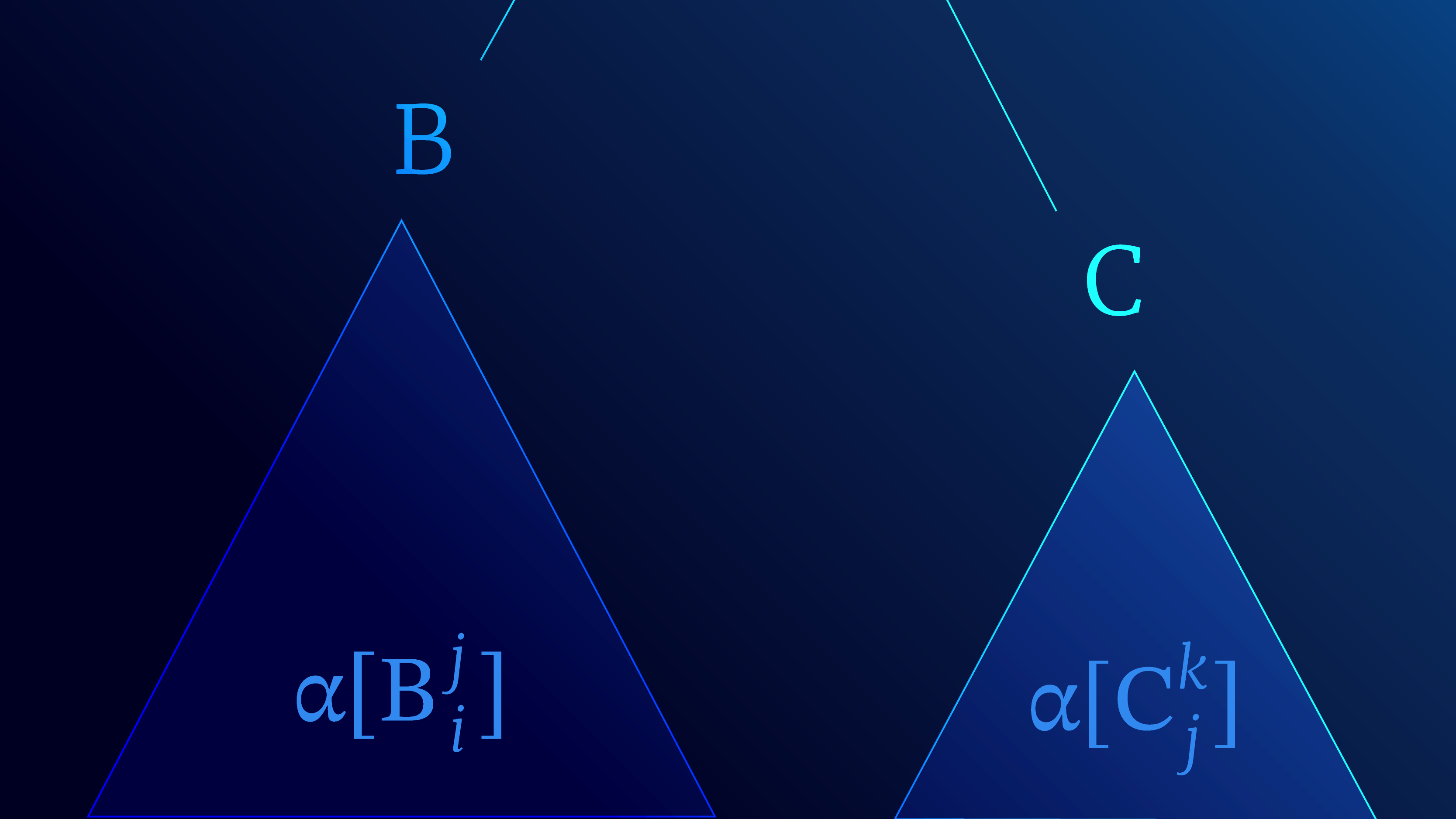
The inside-weight $\alpha[A_i^k]$ corresponds to the sum of all the left and right sub-trees considering all possible split points $j$ and all possible non-terminals B and C (figure 5).

Figure 5. Interpretation of inside weights. The inside weights $\alpha[B_i^j]$ and $\alpha[C_j^k]$ correspond to the total weights of
all the sub-trees that feed upwards into non-terminals $B$ and $C$ respectively (shaded regions). These are used to update the inside weights $\alpha[A_i^k]$ for non-terminal A (see equation 4).
Weighted Parsing
In the previous section, we saw that we could transform the CYK recognition algorithm into the inside algorithm, by just changing the underlying semiring. With his small adjustment, we showed that we can compute the partition function (sum of weights of all tree derivations) in polynomial time. In this section, we apply a similar trick to weighted parsing.
Recall that the partition function $Z$ was defined as the sum of all possible derivations:
\begin{eqnarray} Z &=& \sum_{T \in \mathcal{T}[\mathbf{w}]} \mbox{G}[T] \nonumber \\ &=& \sum_{T \in \mathcal{T}[\mathbf{w}]} \prod_{t \in T} \mbox{g}[T_t], \tag{5} \end{eqnarray}
In contrast, weighted parsing aims to find the derivation $T^{*}$ with the highest weight among all possible derivations:
\begin{eqnarray} T^{*} &=& \underset{T \in \mathcal{T}[\mathbf{w}]}{\text{arg} \, \text{max}} \; \left[\mbox{G}[T]\right] \nonumber \\ &=& \underset{T \in \mathcal{T}[\mathbf{w}]}{\text{arg} \, \text{max}} \left[\prod_{t \in T} \mbox{g}[T_t]\right], \tag{6} \end{eqnarray}
where $\mbox{G}[T]$ is the weight of a derivation tree which is computed by taking the product of the weights $\mbox{g}[T_t]$ of the rules.
Once again we will modify the semiring in the CYK algorithm to perform the task. Let us replace the sum-product semiring $\langle\mathbb{R}_{\geq 0} \cup \{+\infty\} , +, \times, 0, 1\rangle$ with the max-product semiring $<\mathbb{R}_{\geq 0} \cup \{+\infty\} , \max[\bullet], \times, 0, 1>$ to find the score of the “best” derivation. This gives us the following algorithm:
0  # Initialize data structure
1  chart[1...n, 1...n, 1...|V|] := 0
2
3  # Use unary rules to find possible parts of speech at pre-terminals
4  for p := 1 to n   # start position
5    for each unary rule A -> w_p
6        chart[1, p, A] := g[A -> w_p]
7
8  # Main parsing loop
9  for l := 2 to n  # sub-sequence length
10    for p := 1 to n-l+1     # start position
11        for s := 1 to l-1   # split width
12            for each binary rule A -> B C
13                chart[l, p, A] = max[chart[l, p, A],
                                     (g[A -> B C] x chart[s, p, B] x chart[l-s,p+s, C]]
14
15  return chart[n, 1, S]
The differences from the CYK recognition algorithm are colored in green, and the single difference from both the inside algorithm and the CYK recognition algorithm is colored in orange.
Once more, each position $(p,l)$ in the $\texttt{chart}$ represents the sub-sequence that starts at position $p$ and is of length $l$. In the inside algorithm, each position contained a vector with one entry for each of the $|V|$ rules. Each element of this vector contained the sum of the weights of all of the sub-trees which feed into this anchored non-terminal. In this variation, each element contains the maximum weight among all the sub-trees that feed into this anchored non-terminal. Position (n,1) represents the whole string, and so the value $\texttt{chart[n, 1, S]}$ is the maximum weight among all valid parse trees. If this is zero, then there is no valid derivation.
The update rule at line 13 for the weight at $\texttt{chart[l, p, A]}$ now has the following interpretation. For each rule $\texttt{A -> B C}$ and for each possible split $\texttt{s}$ of the data, we multiply the the rule weight $\texttt{g[A -> B C]}$ by the two weights $\texttt{chart[s, p, B]}$ and $\texttt{chart[l-s, p+s, B]}$ associated with the two child sub-sequences. If the result is larger than the current highest value, then we update it. If we are interested in the parse tree itself, then we can store back-pointers indicating which split yielded the maximum value at each position, and traverse backwards to retrieve the best tree.
Worked example
In figure 6 we illustrate worked example of weighted parsing. The algorithm starts by assigning weights to pre-terminals exactly as in figure 3a. The computation of the weights for sub-sequences of length $l=2$ is also exactly as in figure 3b, and the algorithm also proceeds identically for $l=3$ and $l=4$.
The sole difference occurs for the sub-sequence of length $l=5$ at position $p=2$ (figure 6). There are two possible rules that both assign the non-terminal VP to the chart at this position. In the inside algorithm, we calculated the weights of these rules and summed them. In weighted parsing, we store the largest of these weights, and this operation corresponds to the $\mbox{max}[\bullet,\bullet]$ function on line 13 of the algorithm.

Figure 6. Weighted parsing worked example. a) When we get to string length $l=5$, position $p=2$ there are two possible rules that both assign the non-terminal VP to this position, which correspond to the red and blue sub-trees respectively. We calculate the weight for each as normal (rule weight $\times$ left tree weight $\times$ right tree weight), but then assign the maximum of these to the current position. b) Upon completion, the value associated with the start symbol S in the top-left corner is the maximum weight of all the parse trees. By keeping track of which sub-trees contributed to this (i.e, the blue sub-tree rather than the red one), we can retrieve this maximum weighted tree which is the “best” parse of the sentence according to the weighted context-free grammar.
At the end of the procedure, the weight associated with the start symbol at position (6,1) corresponds to the tree with the maximum weight and so is considered the “best”. By keeping track of which sub-tree yielded the maximum weight at each split, we can retrieve this tree which corresponds to our best guess at parsing the sentence.
Summary
We’ve seen that we can add weights to CFGs and replace the $AND, OR$ semiring with $+, \times$ to find the total weight of all possible derivations (i.e. compute the partition function with the inside algorithm). Further more, but we can use $\max, \times$ instead to find the parse tree with the highest weight.
The semirings allow us to unify the CYK recognition, inside, and weighted parsing algorithms by recursively defining the chart entries as:
\begin{equation} \texttt{chart}[A_i^k] = \bigoplus_{B, C, j} \mbox{g}[A \rightarrow B C] \otimes \texttt{chart}[B_i^j] \otimes \texttt{chart}[C_i^k], \tag{7} \end{equation}
where for recognition $\mbox{g}[A \rightarrow B C]$ just returns $\texttt{TRUE}$ for all existing rules.
Readers familiar with graphical models, will no doubt have noticed the similarity between these methods and sum-product and max-product belief propagation. Indeed, we could alternatively have presented this entire argument in terms of graphical models, but the semiring formulation is more concise.
In the final part of this blog, we will consider probabilistic context-free grammars, which are a special case of weighted-context free grammars. We’ll develop algorithms to learn the weights from (i) a corpus of sentences with known parse trees and (ii) just the sentences. The latter case will lead to a discussion of the famous inside-outside algorithm.
1. If you are wondering why is it “semi”, its because the magnificent rings also have an additive inverse for each element: $x \oplus (-x) = 0$.
News
Meet Turing by Borealis AI, an AI-powered text to SQL database interface
Blog
Tutorial #15: Parsing I context-free grammars and the CYK algorithm
Work with Us!
Impressed by the work of the team? Borealis AI is looking to hire for various roles across different teams. Visit our career page now and discover opportunities to join similar impactful projects!
Careers at Borealis AI