
From traditional Machine Learning models like linear regression to Deep Learning models like transformers, machine learning techniques usually require thousands to millions of examples to learn a new concept. However, in some cases, it may only take a human a couple of examples to gain the same level of knowledge. Is it possible to develop some ML algorithms to achieve similar behaviours? In this tutorial, you will learn the progress researchers have made in the few-shot and meta-learning area and how it helps close the gap we mentioned above.
What is Few-shot Learning?
Few-shot learning refers to the ability of learning new concepts by training machine learning models with only a few examples. It can be very helpful in cases where:
• One wants to avoid data hunger due to the high resource and computation cost of training a model with large amount of data.
• It’s nearly impossible to have access to large amounts of labeled data due to the nature of the problem or privacy concerns.
• The solution will be used in scenarios where the model needs to adapt quickly to new tasks or domains before a large amount of labeled data is collected.
Few-shot Learning Problem Setup
Few-shot learning is usually studied using N-way-K-shot classification.
N-way-K-shot classification aims to discriminate between N classes with K examples of each. A typical problem size might be to discriminate between N = 10 classes with only K = 5 samples from each to train from.
How to achieve Few-shot Learning?
We cannot train a classifier using conventional methods here; any modern classification algorithm will depend on far more parameters than there are training examples and will generalize poorly. If the data is insufficient to constrain the problem, then one possible solution is to gain experience from other similar problems. To this end, most approaches to achieve few-shot learning fall in the meta-learning area.
What is Meta-learning?
Meta-learning, or learning to learn, performs the learning through multiple training episodes. During this process, it learns how to improve the learning algorithm itself. Hence, it has demonstrated better performance at generalization, especially when a limited amount of data is given.
The meta-learning framework for few-shot learning
In the classical learning framework, we learn how to classify from training data and evaluate the results using test data. In the meta-learning framework, we learn how to learn to classify given a set of training tasks and evaluate using a set of test tasks (figure 1); In other words, we use one set of classification problems to help solve other unrelated sets.
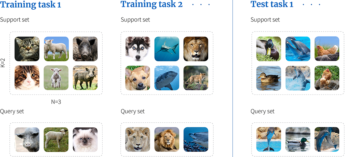
Figure 1. Meta-learning framework. An algorithm is trained using a series of training tasks. Here, each task is a 3-way-2-shot classification problem because each training task contains a support set with three different classes and two examples of each. During training the cost function assesses performance on the query set for each task in turn given the respective support set. At test time, we use a completely different set of tasks, and evaluate performance on the query set, given the support set. Note that there is no overlap between the classes in the two training tasks {cat, lamb, pig}, {dog, shark, lion} and between those in the test task {duck, dolphin, hen}, so the algorithm must learn to classify image classes in general rather than any particular set.
Here, each task mimics the few-shot scenario, so for N-way-K-shot classification, each task includes $N$ classes with $K$ examples of each. These are known as the support set for the task and are used for learning how to solve this task. In addition, there are further examples of the same classes, known as a query set, which are used to evaluate the performance on this task. Each task can be completely non-overlapping; we may never see the classes from one task in any of the others. The idea is that the system repeatedly sees instances (tasks) during training that match the structure of the final few-shot task but contain different classes.
At each step of meta-learning, we update the model parameters based on a randomly selected training task. The loss function is determined by the classification performance on the query set of this training task, based on knowledge gained from its support set. Since the network is presented with a different task at each time step, it must learn how to discriminate data classes in general rather than a particular subset of classes.
To evaluate few-shot performance, we use a set of test tasks. Each contains only unseen classes that were not in any of the training tasks. For each, we measure performance on the query set based on knowledge of their support set.
Approaches to meta-learning
Approaches to meta-learning are diverse, and there is no consensus on the best approach. However, there are three distinct families, each of which exploits a different type of prior knowledge:
Prior knowledge about similarity: We learn embeddings in training tasks that tend to separate different classes even when they are unseen.
Prior knowledge about learning: We use prior knowledge to constrain the learning algorithm to choose parameters that generalize well from few examples.
Prior knowledge of data: We exploit prior knowledge about the structure and variability of the data and this allows us to learn viable models from few examples.
An overview these methods can be seen in figure 2. In this review, we will consider each family of methods in turn.
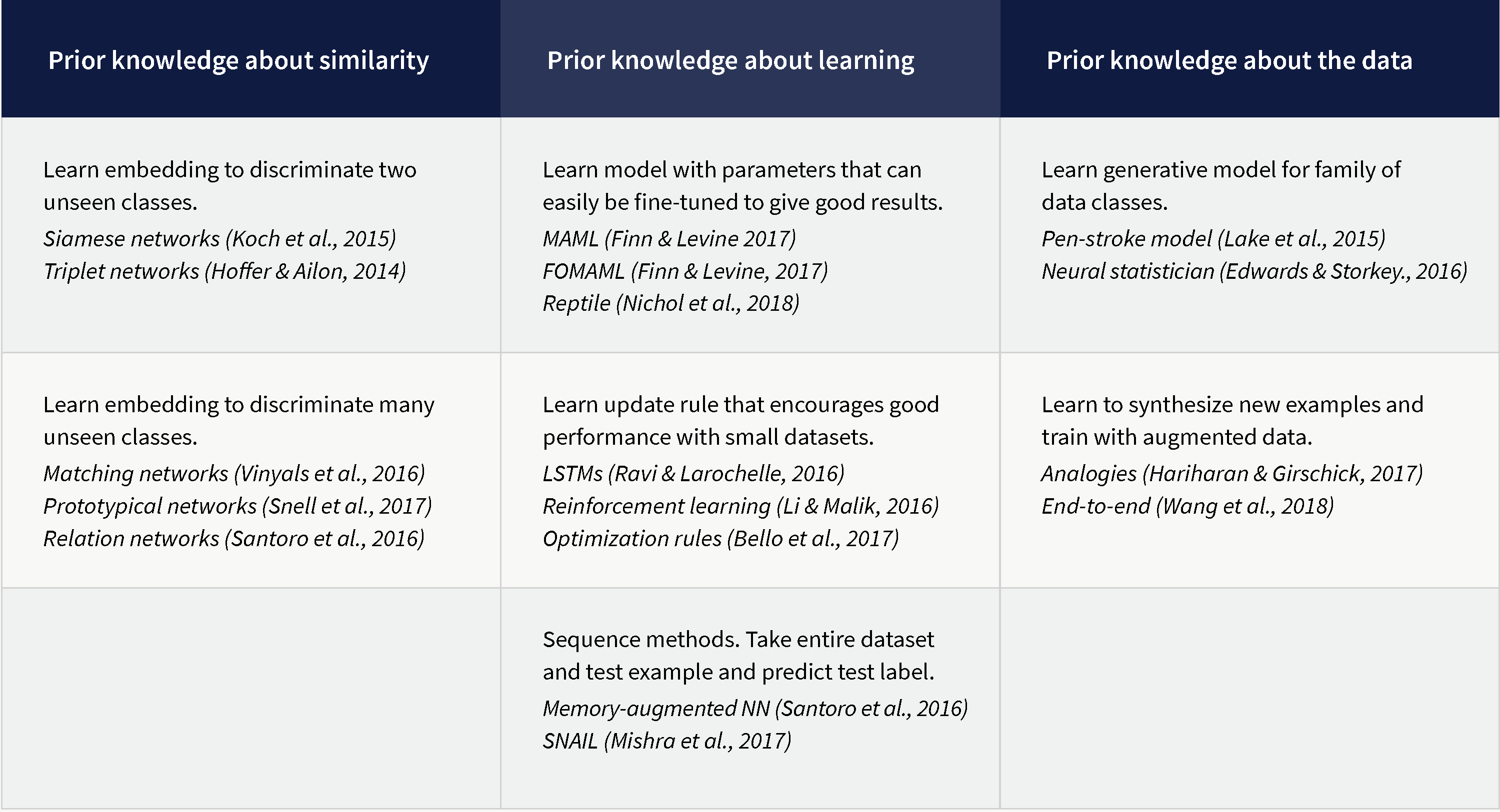
Figure 2. Few-shot learning methods can be divided into three families. The first family learns prior knowledge about the similarity and dissimilarity of classes (in the form of embeddings) from training tasks. The second family exploits prior knowledge about how to learn that it has garnered from training tasks. The third family exploits prior knowledge about the data and its likely variation that is has learned from training tasks.
Prior knowledge of similarity

Figure 3. Pairwise comparators. a) Siamese networks take two examples $\mathbf{x}_{a}$ and $\mathbf{x}_{b}$ and return the probability $Pr(y_{a}=y_{b})$ that they are the same class. They do this by passing each example through an identical network (hence Siamese) and then using the pairwise difference between the embeddings as the basis of the decision. b) Triplet networks take two examples of the same class $\mathbf{x}_{a}$ and $\mathbf{x}_{+}$ and one of a different class $\mathbf{x}_{-}$ and pass all three through identical networks to create three embeddings. The triplet loss encourages the embeddings of examples from the same class to be closer together than those from different classes. c) In the test phase for triplet networks, we pass two examples $\mathbf{x}_{a}$ and $\mathbf{x}_{b}$ through the same network and judge whether they come from the same class or not based on the distance.
This family of algorithms aims to learn compact representations (embeddings) in which the data vector is mostly unaffected by intra-class variations but retains information about class membership. Early work focused on pairwise comparators, which aim to judge whether two data examples are from the same or different classes, even though the system may not have seen these classes before. Subsequent research focused on multi-class comparators which allow the assignment of new examples to one of several classes.
Pairwise comparators
Pairwise comparators take two examples and classify them as either belonging to the same or different classes. This differs from the standard N-way-K-shot configuration and does not obviously map onto the above description of meta-learning although as we will see later, there is, in fact a close relationship.
Siamese networks
(Koch et al. (2015) trained a model that outputs the probability $Pr(y_a=y_{b})$ that two data examples $\mathbf{x}_{a}$ and $\mathbf{x}_{b}$ belong to the same class (figure 3a). The two examples are passed through identical multi-layer neural networks (hence Siamese) to create two embeddings. The component-wise absolute distance between the embeddings is computed and passed to a subsequent comparison network that reduces this distance vector to a single number. This is passed through a sigmoidal output for classification as being the same or different with a cross-entropy loss.
During training, each pair of examples are randomly drawn from a super-set of training classes. Hence, the system learns to discriminate between classes is general rather than two classes in particular. In testing, completely different classes are used. Although this does not have the formal structure of the N-way-K-shot task, the spirit is similar.
Triplet networks
Triplet networks (Hoffer & Ailon 2015) consist of three identical networks that are trained by triplets $\{\mathbf{x}_{+},\mathbf{x}_{a},\mathbf{x}_{-}\}$ of the form (positive, anchor, negative). The positive and anchor samples are from the same class, whereas the negative sample is from a different class. The learning criterion is triplet loss which encourages the anchor to be closer to the positive example than it is to the negative example in the embedding space (figure 3b). Hence it is based on two pairwise comparisons.
After training, the system can take two examples and establish whether they are from the same or different classes, by thresholding the distance in the learned embedding space. This was employed in the context of face verification by Schroff et al. (2015). This line of work is part of a greater literature on learning distance metrics (see Suarez et al. 2018 for an overview).
Multi-class comparators
Pairwise comparators can be adapted to the N-way-K-shot setting by assigning the class for an example in the query set based on its maximum similarity to one of the examples in the support set. However, multi-class comparators attempt to do the same thing in a more principled way; here the representation and final classification are learned in an end-to-end fashion.
In this section, we’ll use the notation $\mathbf{x}_{nk}$ to denote the $k$th support example from the $n$th class in the N-Way-K-Shot classification task, and $y_{nk}$ to denote the corresponding label. For simplicity, we’ll assume there is a single query example $\hat{\mathbf{x}}$ and the goal is to predict the associated label $\hat{y}$.
Matching Networks
Matching networks (Vinyals et al. 2016) predict the one-hot encoded query-set label $\hat{\mathbf{y}}$ as a weighted sum of all of the one-hot encoded support-set labels $\{\mathbf{y}_{nk}\}_{n,k=1}^{NK}$. The weight is based on a computed similarity $a[\hat{\mathbf{x}},\mathbf{x}_{nk}]$ between the query-set data $\hat{\mathbf{x}}$ and each training example $\{\mathbf{x}_{nk}\}_{n,k=1}^{N,K}$.
\begin{equation} \hat{\mathbf{y}} = \sum_{n=1}^{N}\sum_{k=1}^{K} a[\mathbf{x}_{nk},\hat{\mathbf{x}}]\mathbf{y}_{nk} \tag{1.1}\end{equation}
where the similarities have been constrained to be positive and sum to one.
To compute the similarity $a[\hat{\mathbf{x}},\mathbf{x}_{nk}]$, they pass each support example $\mathbf{x}_{nk}$ through a network $\mbox{ f}[\bullet]$ to produce an embedding and pass the query example $\hat{\mathbf{x}}$ through a different network $\mbox{ g}[\bullet]$ to produce a different embedding. They then compute the cosine similarity between these embeddings (figure 5a)
\begin{equation} d[\mathbf{x}_{nk}, \hat{\mathbf{x}}] = \frac{\mbox{ f}[\mathbf{x}_{nk}]^{T}\mbox{ g}[\hat{\mathbf{x}}]} {||\mbox{ f}[\mathbf{x}_{nk}]||\cdot||\mbox{ g}[\hat{\mathbf{x}}]||}, \tag{1.2}\end{equation}
and normalize using a softmax function:
\begin{equation} a[\hat{\mathbf{x}}_{nk},\mathbf{x}] = \frac{\exp[d[\mathbf{x}_{nk},\hat{\mathbf{x}}]]}{\sum_{n=1}^{N}\sum_{k=1}^{K}\exp[d[\mathbf{x}_{nk},\hat{\mathbf{x}}]]}. \tag{1.3}\end{equation}
to produce positive similarities that sum to one. This system can be trained end to end for the N-way-K-shot learning task.1 At each learning iteration, the system is presented with a training task; the predicted labels are computed for the query set (the calculation is based on the support set) and the loss function is the cross entropy of the ground truth and predicted labels.
Matching networks compute similarities between the embeddings of each support example and the query example. This has the disadvantage that the algorithm is not robust to data imbalance; if there are more support examples for some classes than others (i.e., we have departed from the N-way-K-shot scenario), the ones with more frequent training data may dominate.
Prototypical Networks
Prototypical networks (Snell et al. 2017) are robust to data imbalance by construction; they average the embeddings $\{\mathbf{z}_{nk}\}_{k=1}^{K}$ of the examples for class $n$ to compute their mean embedding or prototype $\mathbf{p}_{n}$. They then use the similarity between each prototype and the query embedding (figures 4 and 5 b) as a basis for classification.
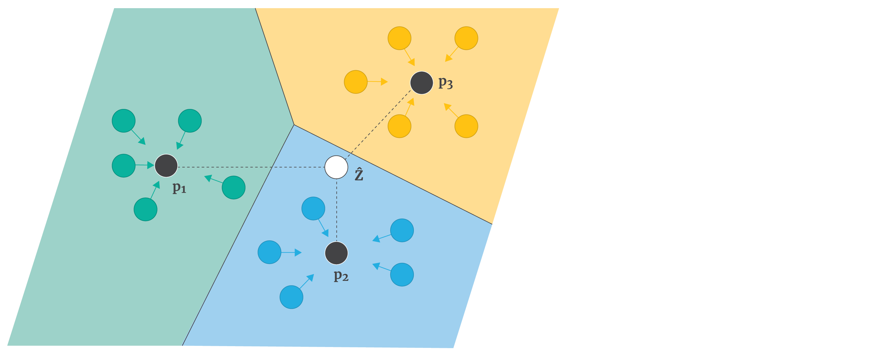
Figure 4. Prototypical networks. The support examples $\mathbf{x}_{nk}$ are all mapped to the embedding space to create embedding $\mathbf{z}_{nk}$ (coloured circles). All of the embeddings for class $k$ are averaged to create a prototype $\mathbf{p}_{n}$. To classify query examples $\hat{\mathbf{x}}$, we first compute its embedding $\hat{\mathbf{z}}$ and then base the decision on the relative distance to the prototypes.
The similarity is computed as a negative multiple of the Euclidean distance (so that larger distances now give smaller numbers). They pass these similarities to a softmax function to give a probability over classes. This model effectively learns a metric space where the average of a few examples of a class is a good representation of that class, and class membership can be assigned based on distance.
They noted that (i) the choice of distance function is vital as squared Euclidean distance outperformed cosine distance, (ii) having a higher number of classes in the support set helps to achieve better performance, and (iii) the system works best when the support size of each class is matched in the training and test tasks.
Ren et al. (2018) extended this system to take advantage of additional unlabeled data, which might be from the test task classes or from other distractor classes. Oreshkin et al. (2018) extended this approach by learning a task-dependent metric on the feature space so that the distance metric changes from place to place in the embedding space.
Relation Networks
Matching networks and prototypical networks both focus on learning the embedding and comparing examples using a pre-defined metric (cosine and Euclidean distance, respectively). Relation networks (Santoro et al. 2016) also learn a metric for comparison of the embeddings (figure 5c). Similarly to prototypical networks, the relation network averages the embeddings of each class in the support set together to form a single prototype. Each prototype is then concatenated with the query embedding and passed to a relation module. This is a learnable non-linear operator that produces a similarity score between 0 and 1 where 1 indicates that the query example belongs to this class prototype. This approach is clean and elegant and can be trained end-to-end.
Holistic view of pairwise comparators and mutli-class comparators
All of the pairwise and multi-class comparators are closely related to one another. Each learns an embedding space for data examples. In matching networks, there are different embeddings for support and query examples, but in the other models, they are the same. For prototypical networks and relation networks, multiple embeddings from the same class are averaged to form prototypes. Distances between support set embeddings/prototypes and query set embeddings are computed using either pre-determined distance functions such as Euclidean or cosine distance (triplet networks, matching networks, prototypical networks) or by learning a distance metric (Siamese networks and relation networks).

Figure 5. Multi-class comparators. a) Matching networks compute separate embeddings for support examples (here $\mathbf{x}_{11},\mathbf{x}_{12},\mathbf{x}_{21},\mathbf{x}_{22}$) and the query example $\hat{\mathbf{x}}$. Here $\mathbf{x}_{nk}$ is the $k$th example from the $n$th class. They compute the cosine similarity between each support embedding and the the query embedding, and then use these similarities to choose the class. This has the disadvantage that if there are many more examples of one class than the others, the relatively abundant class may be chosen too frequently. b) Prototypical networks embed the query and support examples using the same network, but average together support embeddings to make prototypes for each class, and so it doesn’t matter if the numbers are unbalanced. The Euclidean distance between query embeddings and prototypes is used to support classification. c) Relation networks replace this Euclidean distance with a learned non-linear distance metric.
The multi-class networks have the advantage that they can be trained end-to-end for the N-way-K-shot classification task. This is not true for the pairwise comparators which are trained to produce a similarity or distance between pairs of data examples (which could itself subsequently be used to support multi-class classification).
Although it is not obvious how the pairwise comparators map to the meta-learning framework, it is possible to consider their data as consisting of minimal training and test tasks. For Siamese networks, each pair of examples is a training task consisting of one support example and one query example, where their classes may not necessarily match. For triplet networks, there are two support examples (from different classes) and one query example (from one of the classes).
Recent Advancements in meta-learning using prior knowledge of similarity
Beyond the above classical works, many new algorithms have been proposed by researchers to improve few-shot learning based on prior knowledge of similarity. Below, we listed a couple of works:
TADAM: Task dependent adaptive metric for improved few-shot learning (Oreshkin et al. 2018) – Introduced learnable parameters for metric scaling to replace static similarity metrics like Euclidian distance and cosine similarity metric. It also added a task embedding network and auxiliary co-learning tasks on top of Prototypical networks to improve the learning performance.
RelationNet2: Deep Comparison Columns for Few-Shot Learning (Zhang et al. 2018) – Improves the work of RelationNet by learning relations based on different levels of feature representation simultaneously instead of just based on the final layer of embedding. Also, instead of learning discriminate features, it learns a distribution with parameterized Gaussian noise to help with model generalization.
Cross attention network for few-shot classification (Hou et al. 2019) – Different from existing methods, after getting the embedding representation of the support set and query example independently, they introduced a Cross Attention Module (CAM) to model the semantic relevance between the two before sending it for downstream similarity-based classification.
Self-supervised learning for few-shot image classification (Chen et al. 2019) – Argued that the embedding learned through supervised learning is the bottleneck of the few-shot learning methods due to the small size of the support set. They propose to train a more generalized embedding network with self-supervised learning, which provides a more robust representation for downstream tasks by learning from the data itself.
Recent surveys comparing few-shot learning models
Comprehensive study and performance comparison of a range of few-shot learning models can be found in recent surveys:
[1] Wang, Yaqing, et al. “Generalizing from a few examples: A survey on few-shot learning.” ACM computing surveys (csur) 53.3 (2020): 1-34.
[2] Parnami, Archit, and Minwoo Lee. “Learning from few examples: A summary of approaches to few-shot learning.” arXiv preprint arXiv:2203.04291 (2022).
Key learnings and future reading
In part I of this tutorial, we have described few-shot learning and meta-learning and introduced a taxonomy of methods, including prior knowledge about similarity, prior knowledge about algorithm and priory of data. We discussed pairwise comparators, including Siamese Networks and Triplet Networks. We also introduced multi-class comparators, including Matching Networks, Prototypical Networks and Relation Networks. Both types of comparators use a series of training tasks to learn prior knowledge about the similarity and dissimilarity of classes that can be exploited for future few-shot tasks. This knowledge takes the form of data embeddings that reduce within-class variance relative to between-class variance and hence make it easier to learn from just a few data points.
Interested in further expanding your knowledge of few-shot learning and meta-learning? In part II of this tutorial series, we dive deeper into few-shot learning and meta-learning. We’ll discuss methods that incorporate prior knowledge about how to learn models and that incorporate prior knowledge about the data itself.
Related Content
-
Tutorial #3: few-shot learning and meta-learning II
Tutorial #3: few-shot learning and meta-learning II
S. Prince, L. S. Ghoraie, and W. Zi.
-
Adaptive Models of Non-Stationary Dynamics in Capital Markets
Adaptive Models of Non-Stationary Dynamics in Capital Markets
S. Liu, and A. Lehrmann.
-
Latent Bottlenecked Attentive Neural Processes
Latent Bottlenecked Attentive Neural Processes
L. Feng, H. Hajimirsadeghi, Y. Bengio, and M. O. Ahmed. International Conference on Learning Representations (ICLR), 2023
Work with us!

Impressed by the work of the team?
Borealis AI is looking to hire for various roles across different teams. Visit our career page now to find the right role for you and join our team!