In Part I of this tutorial, we introduced context-free grammars and the CYK recognition algorithm. In Part II we discussed weighted context-free grammars in which each rule from the grammar is assigned a non-negative weight, and the weight of a parse tree is a product of its component rules. This led to the inside algorithm (which computed the sum of the weights of all valid parse trees) and the weighted parsing algorithm (which retrieved the tree with the highest weight).
In this final post, we consider probabilistic context-free grammars or PCFGs, which are are a special case of WCFGs. They are featured more than WCFGs in the earlier statistical NLP literature and in most teaching materials. As the name suggests, they replace the rule weights with probabilities. We will treat these probabilities as model parameters and describe algorithms to learn them for both the supervised and the unsupervised cases. The latter is tackled by expectation-maximization and leads us to develop the inside-outside algorithm which computes the expected rule counts that are required for the EM updates.
Probabilistic context-free grammars
PCFGs are the same as WCFGs except that the weights are constrained; the weights of all rules with the same non-terminal on the left-hand side must be non-negative and sum to one:
\begin{equation} \sum_{\alpha} \mbox{g}[\text{A} \rightarrow \alpha] = 1. \tag{1}\end{equation}
For example, we might have three rules with VP on the left-hand side: $\text{VP} \rightarrow \text{NP}$, $\text{VP} \rightarrow \text{NN}$ and $\text{VP} \rightarrow \text{PN}$. For a PCFG, this implies that:
\begin{equation} \mbox{g}[\text{VP} \rightarrow \text{NP}]+\mbox{g}[\text{VP} \rightarrow \text{NN}]+\mbox{g}[\text{VP} \rightarrow \text{PN}]= 1. \tag{2}\end{equation}
The rule weights are now probabilities and the weight $\mbox{G}[T]$ of an entire tree is the product of these probabilities. The tree weight $\mbox{G}[T]$ can hence be interpreted as the probability $Pr(T)$ of the tree:
\begin{eqnarray}\label{eq:tree_like} Pr(T) &=& \mbox{G}[T]\nonumber \\ &=& \prod_{t\in T} \mbox{g}[T_{t}]\nonumber \\ &=& \prod_{A}\prod_{\alpha} \mbox{g}[\text{A} \rightarrow \alpha]^{\mbox{f}_{\text{A}\rightarrow\alpha}[T]} \tag{3}\end{eqnarray}
where the function $f_{\text{A} \rightarrow \alpha}[T]$ counts the number of times $\text{A} \rightarrow \alpha$ appears in tree $T$.
Marginal, joint, and conditional distributions
PCFGs define a joint distribution $Pr(T,\mathbf{w})$ of trees $T$ and sentences $\mathbf{w}$. The probability of a sentence $Pr(\mathbf{w})$ can be computed through marginalization:
\begin{equation}\label{eq:parse_marginal} Pr(\mathbf{w}) = \sum_{T\in \mathcal{T}[\mathbf{w}]} Pr(\mathbf{w}, T), \tag{4}\end{equation}
where $\mathcal{T}[\mathbf{w}]$ is the set of all parse trees that are compatible with the observed sentence $\mathbf{w}$.
The conditional probability of the sentence $Pr(\mathbf{w}|T)$ given the tree is just $1$, because the tree yields $\mathbf{w}$ (i.e., the tree deterministically produces the words). It follows that the joint distribution is:
\begin{equation}\label{eq:parsing_joint} Pr(T,\mathbf{w}) = Pr(\mathbf{w}|T) Pr(T) = Pr(T). \tag{5}\end{equation}
However, the conditional probability $Pr(T|\mathbf{w})\neq 1$ in general. When a sentence is ambiguous, there are multiple trees that can produce the same words. For PCFGs, the weighted parsing algorithm returns the tree with the maximum conditional probability, and the inside algorithm returns the marginal probability of the sentence (equation 4).
Generating text from PCFGs
PCFGs are a generative approach to syntactic analysis in that they represent joint distributions over sentences and parse trees. They can also be used to sample random sentences: we start by drawing a sample from all of the rules $\text{S} \rightarrow \alpha$ with the start token $S$ on the left hand side according to the probabilities $g[\text{S}\rightarrow \alpha]$. For example, we might draw $\text{S}\rightarrow\text{NP VP}$. Then we draw samples from rules with $\text{NP}$ and $\text{VP}$ on the left hand-side respectively. The process continues until it draws terminal symbols (i.e., words) in every branch of the tree and no non-terminals remain at the leaves.
Parameter estimation: supervised
We now turn our attention to learning the rule probabilities for a PCFG. In this section we’ll consider the supervised case where we have a treebank (i.e, a set of sentences annotated with trees). We ‘ll show that we can estimate the probabilities using a simple counting procedure. In subsequent sections, we’ll consider the unsupervised case, where we must estimate the weights based on the sentences alone.
To learn the parameters of a PCFG from a treebank, we optimize the total log likelihood $L$ of the $I$ observed trees:
\begin{equation} L = \sum_{i=1}^{I}\sum_{A} \sum_{\alpha} f_{\text{A}\rightarrow\alpha}[T_{i}]\log[\mbox{g}[\text{A} \rightarrow \alpha]]. \tag{6}\end{equation}
with respect to the rule probabilities $g[\text{A} \rightarrow \alpha]$. The first sum is over the training examples, the second over the left hand side of the rules and the third over the right-hand side. The function $f_{\text{A} \rightarrow \alpha}[T_{i}]$ counts the number of times rule $\text{A} \rightarrow \alpha$ appears in tree $T_{i}$.
To ensure that the result of this optimization process is a valid PCFG, we must also add a set of constraints that ensure that all rules with the same left-hand side sum to one:
\begin{equation} \sum_{\alpha} \mbox{g}[\text{A} \rightarrow \alpha] = 1\hspace{1cm}\forall \mbox{A}\in\mathcal{V}.\tag{7}\end{equation}
Taking just the terms with A on the left hand side, and adding a Lagrange multiplier that enforces this constraint we have:
\begin{equation} L_{A}^{\prime} = \sum_{i=1}^{I}\sum_{\alpha} f_{\text{A}\rightarrow\alpha}[T_{i}]\log[\mbox{g}[\text{A} \rightarrow \alpha]]+\lambda\left(\sum_{\text{A}}g[\text{A} \rightarrow \alpha] – 1\right). \tag{8}\end{equation}
We then take derivatives with respect to each rule $g[\text{A} \rightarrow \alpha]$ and the Lagrange multiplier $\lambda$ and set the resulting expressions to zero. This yields a set of equations which can be re-arranged to provide the maximum likelihood estimator for a given rule $\mbox{g}[\text{A} \rightarrow \text{B} \text{C}]$:
\begin{equation}\label{eq:treebank_ml} \mbox{g}[\text{A} \rightarrow \text{B} \text{C}] = \frac{\sum_i^I f_{\text{A} \rightarrow \text{B} \text{C}}[T_i]}{\sum_i^I \sum_{\alpha} f_{\text{A}, \rightarrow \alpha}[T_i]}, \tag{9}\end{equation}
where the numerator counts the number of times A is re-written to BC and the denominator counts the number of times it is re-rewritten to anything. See Chi and Geman (1998) for further details.
Worked code example
We’ll now provide some code snippets that use a treebank to estimate the parameters of a PCFG using the above method. In treebanks the constituency trees are usually represented in a bracket notation. For example, the legendary first sentence from the Penn Treebank1 is Pierre Vinken, 61 years old, will join the board as a non-executive director Nov. 29. with associated tree:
( (S
    (NP-SBJ
      (NP (NNP Pierre) (NNP Vinken) )
      (, ,)
      (ADJP
        (NP (CD 61) (NNS years) )
        (JJ old) )
      (, ,) )
    (VP (MD will)
      (VP (VB join)
        (NP (DT the) (NN board) )
        (PP-CLR (IN as)
          (NP (DT a) (JJ nonexecutive) (NN director) ))
        (NP-TMP (NNP Nov.) (CD 29) )))
    (. .) ))
Throughout this section, we’ll provide some Python code snippets that use the NLTK (natural language toolkit) package. We’ll show how to estimate the rule weights from annotated data using NLTK, and then we’ll take a look inside the code to see how it is implemented.
NLTK has the convenient Tree class to make exploration easier:
from nltk.tree import Tree
t = Tree.fromstring("(S (NP I) (VP (V saw) (NP him)))")
To extract a grammar that is useful for parsing we need a to convert the CFG to Chomsky Normal Form:
t.chomsky_normal_form()
We then extract grammar rules from the entire treebank:
productions = []
# Go over all tree-strings
for line in treebank:
    tree = Tree.fromstring(line)
    tree.collapse_unary(collapsePOS = False)
    tree.chomsky_normal_form(horzMarkov = 2)
    productions += tree.productions()
Finally, we learn the weights:
from nltk import Nonterminal
from nltk import induce_pcfg

S = Nonterminal('S')
grammar = induce_pcfg(S, productions)
Now let’s peek into NLTK version 3.6 to see how these estimates are computed:
# Production count: the number of times a given production occurs
pcount = {}

# LHS-count: counts the number of times a given lhs occurs
lcount = {}

for prod in productions:
    lcount[prod.lhs()] = lcount.get(prod.lhs(), 0) + 1
    pcount[prod] = pcount.get(prod, 0) + 1

prods = [
    ProbabilisticProduction(p.lhs(),
                            p.rhs(),
                            prob=pcount[p] / lcount[p.lhs()])
    for p in pcount
]
As expected, this just directly implements equation 13. Given the parameters of the model we can parse a sentence under the induced grammar using the CYK weighted parsing algorithm:
from nltk.parse import ViterbiParser

sent = ['How', 'much', 'is', 'the', 'fish', '?']
parser = ViterbiParser(grammar)
parse = parser.parse(sent)
Parameter estimation: unsupervised
In the previous section, we showed that it is relatively easy to estimate the parameters (rule weights) of PCFGs when we are given a set of sentences with the associated trees. Now we turn our attention to the unsupervised case. Here, we are given the sentences, but not the trees. This is a chicken-and-egg problem. If we knew the rule-weights, then we could perform weighted parsing to find the best fitting trees. Likewise, if we knew the trees, we could estimate the rule weights using the supervised approach above.
In the next section, we’ll introduce some notation and define the cost function for parameter estimation in the unsupervised case. Then we’ll describe two algorithms to optimize this cost function. First we’ll introduce Viterbi training that alternates between finding the best trees for fixed rule weights and updating the rule weights based on these trees. Then, we’ll introduce an expectation maximization (EM) algorithm that follows a similar approach, but takes into account the ambiguity of the parsing procedure.
Cost function
Our goal is to calculate the rule weights $\mbox{g}[\text{A}\rightarrow\text{BC}]$. To make the notation cleaner, we’ll define the vector $\boldsymbol\theta$ to contain the log rule weights, so that the element $\theta_{A \rightarrow BC}$ contains $\log \left[\mbox{g}[A \rightarrow BC]\right]$. We aim to maximize the joint probability of the observed sentences and the associated trees with respect to these parameters:
\begin{equation} \boldsymbol\theta^{*} = \underset{\boldsymbol\theta}{\text{arg}\,\text{max}} \left[\sum_i^I \log\left[Pr(T_{i}, \mathbf{w}_{i}|\boldsymbol\theta)\right]\right] \tag{10}\end{equation}
where $i$ indexes $I$ training examples, each consisting of sentence $\mathbf{w}_{i}$ and associated parse tree $T_{i}$.
Unfortunately, in the unsupervised learning case, we don’t know the associated parse trees. There are two possible solutions to this problem. In Viterbi training, we will simultaneously maximize the likelihood with respect to the parameters $\boldsymbol\theta$ and with respect to the choice of tree $T_{i}$ from the set of valid trees $\mathcal{T}[\mathbf{w}_{i}]$ for each training example $i$:
\begin{equation}\label{eq:parse_viterbi} \boldsymbol\theta^{*} = \underset{\boldsymbol\theta}{\text{arg}\,\text{max}}\left[ \sum_i^I \log\left[\underset{T_{i}\in\mathcal{T}_{i}[\mathbf{w}_{i}]}{\text{arg}\,\text{max}}\left[Pr(T_{i}, \mathbf{w}_{i}|\boldsymbol\theta)\right]\right]\right]. \tag{11}\end{equation}
In the expectation-maximization approach we will marginalize over all the possible trees:
\begin{equation} \boldsymbol\theta^{*} = \underset{\boldsymbol\theta}{\text{arg}\,\text{max}} \left[\sum_i^I \log\left[\sum_{ T_{i}\in\mathcal{T}_{i}[\mathbf{w}_{i}]}Pr(T_{i}, \mathbf{w}_{i}|\boldsymbol\theta)\right]\right]. \tag{12}\end{equation}
To summarize, Viterbi training finds the parameters that maximize the joint likelihood of the sentences and their highest probability parses, while the expectation maximization approach searches for the parameters that maximizes the marginal likelihood of the sentences.
Viterbi training
Viterbi training optimizes the cost function in equation 11 by alternately maximizing over the parameters and fitted trees. More precisely, we first initialize the parameters $\boldsymbol\theta$ to random values. Then we alternate between two steps:
- We run the weighted parsing algorithm for each sentence, $\mathbf{w}_{i}$, to find the tree $T_{i}$ with the highest weight, treating the parameters $\boldsymbol\theta$ as fixed.
- We compute the maximum likelihood estimator for the parameters $\boldsymbol\theta$, treating the parse trees $T_{i}$ as fixed. Since $Pr(T_{i},\mathbf{w}_{i}) = Pr(T_{i})$ (equation 5), this is effectively the same as the supervised algorithm, and the solution is given by:
\begin{equation} \theta_{\text{A} \rightarrow \text{B} \text{C}} = \log\left[ \frac{\sum_i^I f_{\text{A} \rightarrow \text{B} \text{C}}[T_i]}{\sum_i^I \sum_\alpha f_{\text{A} \rightarrow \alpha}[T_i]}\right], \tag{13}\end{equation}
where the function $f_{\text{A} \rightarrow \text{B} \text{C}}[T_i]$ counts the number of times $\text{A} \rightarrow \text{B} \text{C}$ appears in tree $T_i$ and $\sum_\alpha f_{\text{A} \rightarrow \alpha}[T_i]$ counts the number of times that $\text{A}$ is re-written to anything in tree $T_{i}$.
Expectation-maximization
Now let’s turn our attention to the expectation maximization (EM) approach which is somewhat more complicated. Recall that we want to maximize the cost function:
\begin{equation} \boldsymbol\theta^{*} = \underset{\boldsymbol\theta}{\text{arg}\,\text{max}} \left[\sum_i^I \log\left[\sum_{ T_{i}\in\mathcal{T}_{i}[\mathbf{w}_{i}]}Pr(T_{i}, \mathbf{w}_{i}|\boldsymbol\theta)\right]\right]. \tag{14}\end{equation}
We’ll present a brief overview of the EM method in an abstract form. Then we’ll map this to our use case. We’ll find expressions for the E-Step and the M-Step respectively. The expression for the M-Step will contain terms that are expected rule counts. We’ll show that we can find these by taking the derivative of the log partition function. This will finally lead us to the inside-outside algorithm which computes these counts.
EM algorithm overview
The EM algorithm is a general tool for maximizing cost functions of the form:
\begin{equation} \boldsymbol\theta^{*} = \underset{\boldsymbol\theta}{\text{arg}\,\text{max}} \left[\sum_i^I \log\left[\sum_{h_{i}}Pr(h_{i}, \mathbf{w}_{i}|\boldsymbol\theta)\right]\right], \tag{15}\end{equation}
where $h_{i}$ a hidden (i.e., unobserved) variable associated with observations $\mathbf{w}_{i}$.
The EM algorithm alternates between the expectation step (E-step) and the maximization step (M-step). In the E-step, we consider the parameters $\boldsymbol\theta$ to be fixed and compute the posterior distribution $Pr(h_{i}|\mathbf{w}_{i},\boldsymbol\theta)$ over the hidden variables $h_{i}$ for each of the $I$ examples using Bayes’ rule:
\begin{equation} Pr(h_{i}|\mathbf{w}_{i},\boldsymbol\theta) = \frac{Pr(h_{i}, \mathbf{w}_{i}|\boldsymbol\theta)}{\sum_{h_{i}}Pr(h_{i}, \mathbf{w}_{i}|\boldsymbol\theta)}. \tag{16}\end{equation}
In the M-step we update the parameters using the rule:
\begin{eqnarray}\boldsymbol\theta &=&\underset{\boldsymbol\theta}{\text{arg}\,\text{max}}\left[\sum_i^I \sum_{h_{i}}Pr(h_{i}|\mathbf{w}_{i},\boldsymbol\theta^{old})\log\left[Pr(h_{i}, \mathbf{w}_{i}|\boldsymbol\theta)\right]\right]\nonumber \\&=&\underset{\boldsymbol\theta}{\text{arg}\,\text{max}}\left[\sum_i^I \mathbb{E}_{h_{i}}\left[\log\left[Pr(h_{i}, \mathbf{w}_{i}|\boldsymbol\theta)\right]\right]\right] \tag{17}\end{eqnarray}
where the expectation is calculated with respect to the distribution that we computed in the E-Step and $\boldsymbol\theta^{old}$ denotes the previous parameters that were used in the E-Step.
It is not obvious why the EM update rules maximize the cost function in equation 15, but this discussion is beyond the scope of this tutorial. For more information consult chapter 7 of this book.
EM algorithm for estimating rule weights
Now let’s map the EM algorithm back to our use case. Here, the choice of the unknown underlying parse tree $T_{i}$ is the hidden variable, and we also have for our case $Pr(\mathbf{w}_{i},T_{i}) = Pr(T_{i})$ (equation 5). This gives us the E-Step:
\begin{eqnarray} Pr(T_{i}|\mathbf{w}_{i},\boldsymbol\theta) = \frac{Pr(T_{i}|\boldsymbol\theta)}{\sum_{T_{i}\in\mathcal{T}[\mathbf{w}]}Pr(T_{i}|\boldsymbol\theta)}, \tag{18}\end{eqnarray}
and M-Step:
\begin{eqnarray}\label{eq:tree_m_step}\boldsymbol\theta^{t+1} &=&\underset{\boldsymbol\theta}{\text{arg}\,\text{max}}\left[\sum_i^I \mathbb{E}_{T_{i}}\left[\log\left[Pr(T_{i}|\boldsymbol\theta)\right]\right]\right], \tag{19}\end{eqnarray}
where this expectation is with respect to the posterior distribution $Pr(T_{i}|\mathbf{w}_{i},\boldsymbol\theta^{old})$ that was calculated in the E-Step. The maximization in the M-Step is subject to the usual PCFG constraints that the weights of all the rules mapping from a given non-terminal $\text{A}$ must sum to one:
\begin{equation}\label{eq:tree_m_step_constraint} \sum_{\alpha}\exp\left[\theta_{A\rightarrow\alpha}\right] = 1. \tag{20}\end{equation}
We’ll now consider each of those steps in more detail.
E-Step
Recall, that in the E-Step we wish to compute the posterior distribution $Pr(T|\mathbf{w},\boldsymbol\theta)$ over the parse trees $T$ for each sentence $\mathbf{w}$ given the current parameters $\boldsymbol\theta$:
\begin{eqnarray}\label{eq:E-step_parsing} Pr(T|\mathbf{w},\boldsymbol\theta) = \frac{Pr(T|\boldsymbol\theta)}{\sum_{T\in\mathcal{T}[\mathbf{w}]}Pr(T|\boldsymbol\theta)} \tag{21}\end{eqnarray}
For a PCFG, the conditional probability in the numerator is just the product of the weights in the tree and the denominator is the partition function $Z$. Let’s derive an expression for the numerator:
\begin{align} \tag{definition of cond prob}
Pr(T|\boldsymbol\theta^{[t]}) &=\prod_{t \in T} \mbox{g}[T_t]) \\
\tag{log-sum-exp}
&= \exp \left[\sum_{t \in T} \log \left[\mbox{g}[T_t]\right] \right] \\
\tag{parameter notation}
&= \exp \left[\sum_{t \in T} \theta_{T_t} \right] \\
\tag{rule counts}
&= \exp \left[\sum_{r \in R} f_r[T] \cdot \theta_{r} \right]\\
\tag{vectorized}
&= \exp \left[\mathbf{f}^{T} \boldsymbol\theta \right],
\end{align}
where $\mathbf{f}^{T}$ is a $|\mathcal{R}|\times 1$ vector in which the $r^{th}$ entry corresponds to the number of times that rule $R$ occurs in the tree and $\boldsymbol\theta$ is a vector of the same size where each entry is the log probability (weight) of that rule.
Armed with this new formulation, we can now re-write equation 21 as
\begin{eqnarray}\label{eq:E_Step_parsing_post} Pr(T|\mathbf{w}_{i},\boldsymbol\theta) &=& \frac{\exp \left[\mathbf{f}^{T} \boldsymbol\theta \right]}{\sum_{T\in \mathcal{T}[\mathbf{w}]}\exp \left[\mathbf{f}^{T} \boldsymbol\theta \right]}\nonumber \\ &=& \frac{\exp \left[\mathbf{f}^{T} \boldsymbol\theta \right]}{Z}, \tag{22}\end{eqnarray}
where $Z$ is the partition function that we can calculate using the inside algorithm.
M-Step
In the M-Step, we compute:
\begin{eqnarray}\boldsymbol\theta^{t+1} &=&\underset{\boldsymbol\theta}{\text{arg}\,\text{max}}\left[\sum_i^I \mathbb{E}_{T_{i}}\left[\log\left[Pr(T_{i}|\boldsymbol\theta)\right]\right]\right]\nonumber \\&=& \underset{\boldsymbol\theta}{\text{arg}\,\text{max}}\left[\sum_i^I \mathbb{E}_{T_{i}}\left[\sum_{\text{A}}\sum_{\alpha} \mbox{f}_{\text{A}\rightarrow\alpha}[T_{i}]\theta_{\text{A} \rightarrow \alpha}]\right]\right], \tag{23}\end{eqnarray}
where as usual, the function $\mbox{f}_{\text{A}\rightarrow\alpha}[T_{i}]$ counts how many times the rules $\text{A}\rightarrow\alpha$ is used in tree $T_{i}$.
This is now very similar to the supervised case; we maximize equation 23 subject to the constraint in equation 20 using Lagrange multipliers to yield the update rule:
\begin{eqnarray} \theta_{\text{A} \rightarrow \text{B} \text{C}} = \exp\left[\frac{\sum_i^N \mathbb{E}_{T_i} [\mbox{f}_{\text{A} \rightarrow \text{B} \text{C}}[T_i]]}{\sum_i^N \sum_\alpha \mathbb{E}_{T_i} [\mbox{f}_{\text{A} \rightarrow \alpha}[T_i]]} \right], \tag{24}\end{eqnarray}
where the expectation is computed over the posterior distribution $Pr(T_{i}|\mathbf{w}_{i})$ that we compute in the E-Step. The final expression is the same as the supervised case (equation 13) except that we are now using the log weights $\theta_{\text{A} \rightarrow \text{B} \text{C}}$ and we are taking expectations over the counting functions $\mbox{f}_{\text{A} \rightarrow \alpha}[T_i]]$.
Computing expected counts for M-Step
In this section, we’ll derive an expression for the expected counts $\mathbb{E}_{T_i} [\mbox{f}_{\text{A} \rightarrow \text{B} \text{C}}[T_i]]$ in the M-Step. First, we substitute in the expression for the posterior distribution (equation 22) from the E-Step:
\begin{eqnarray}\mathbb{E}_{T}\left[f_{r}\right]&=& \sum_{T\in \mathcal{T}[\mathbf{w}]}Pr(T|\mathbf{w},\boldsymbol\theta)\cdot f_{r}\nonumber \\&=& \frac{1}{Z}\sum_{T\in \mathcal{T}[\mathbf{w}]}\exp \left[\mathbf{f}^{T} \cdot \boldsymbol\theta \right]\cdot f_{r} \tag{25}\end{eqnarray}
Now we perform some algebraic manipulation of the right hand side:
\begin{eqnarray}\mathbb{E}_{T}\left[f_{r}\right]&=& \frac{1}{Z}\sum_{T\in \mathcal{T}[\mathbf{w}]}\exp \left[\mathbf{f}^{T} \cdot \boldsymbol\theta \right]\cdot f_{r} \nonumber \\&=& \frac{1}{Z}\sum_{T\in \mathcal{T}[\mathbf{w}]}\exp \left[\mathbf{f}_{j}^{T}\boldsymbol\theta \right]\frac{\partial }{\partial \theta_{r}} \mathbf{f}^{T} \cdot \boldsymbol\theta \nonumber \\&=&\frac{1}{Z}\frac{\partial }{\partial \theta_{r}} \sum_{T\in \mathcal{T}[\mathbf{w}]}\exp \left[\mathbf{f}^{T} \boldsymbol\theta \right]\nonumber\\&=& \frac{1}{Z}\frac{\partial Z}{\partial \theta_{r}} \nonumber\\&=& \frac{\partial \log[Z]}{\partial \theta_{r}}. \tag{26}\end{eqnarray}
We see that the expected count for the $r^{th}$ rule is just the derivative of the log partition function $Z$ with respect to the $r^{th}$ log weight $\theta_{r}$, which we calculated with the inside algorithm.
EM algorithm overview
To summarize the EM algorithm, we alternate between computing the expected counts for each rule $\text{A} \rightarrow \text{B} \text{C}$ and sentence $\mathbf{w}_{i}$:
\begin{eqnarray}\mathbb{E_{T_i}}\left[\mbox{f}_{\text{A} \rightarrow \text{B} \text{C}}\right] &=& \frac{\partial \log[Z_{i}]}{\partial \theta_{\text{A} \rightarrow \text{B} \text{C}}}, \tag{27}\end{eqnarray}
and updating the parameters:
\begin{eqnarray} \theta_{\text{A} \rightarrow \text{B} \text{C}} = \exp\left[\frac{\sum_i^N \mathbb{E}_{T_i} [\mbox{f}_{\text{A} \rightarrow \text{B} \text{C}}[T_i]]}{\sum_i^N \sum_\alpha \mathbb{E}_{T_i} [\mbox{f}_{\text{A} \rightarrow \alpha}[T_i]]} \right]. \tag{28}\end{eqnarray}
To do this, we need to know how to compute the derivative of the log partition function. Since the log-partition function is calculated using the inside algorithm, a really simple way to do this is just to use automatic differentiation. We treat the inside algorithm as a differentiable function as we would a neural network and use backpropagation to estimate the derivatives using code similar to: Z = inside(w, $\theta$); log(Z).backward(). This is known as the inside-outside algorithm.
Outside from inside
In the previous section, we argued that we could compute the expected counts by automatic differentiation of the inside algorithm. In this section, we’ll take this one step further; we’ll apply backpropagation by hand to the inside-algorithm, to yield the outside algorithm which directly computes these counts.
Let’s think of the inside-algorithm as a differentiable program. It takes a sentence $\mathbf{w}$ and parameters $\log[g_{r}] = \theta_r$ as input, and returns the partition function $Z$ as output. The code is:
0 # Initialize data structure1 chart[1…n, 1…n, 1…|V|] := 0
2
3 # Use unary rules to find possible parts of speech at pre-terminals
4 for k := 1 to n # start position
5 for each unary rule A -> w_k
6 chart[k-1, k, A] := g(A -> w_k)
7
8 # Sum over binary rules
9 for l := 2 to n # sub-string length
10 for i := 1 to n-l #start point
11 k = i + l #end point
11 for j := i + 1 to k-1 # mid point
12 for each binary rule A -> B C
13 chart[i, k, A] += g[A -> B C] x
chart[i, j, B] x
chart[j, k, C]
14
15 return chart[0, n, S]
Notice that we have changed the indexing in the loops from our original presentation. This will make the notation less cumbersome. In this notation, the chart is indexed so that chart[i, k, A] contains the inside weights $\alpha[\text{A}_i^k]$ that represent the total weight of all the feasible trees in the sub-sequence from position $i$ to position $k$.
Now consider what happens when we call log(Z).backward(). In the original inside algorithm, we worked from the leaves of the parse tree up to the root where the partition function was computed. When we backpropagate, we reverse this order of operations and work from the root downwards. We’ll now work backwards through the inside algorithm and discuss each part in turn.
Main loop: Based on this intuition we can already sketch the loop structure going backwards from largest constituent to smallest:
1 # Main parsing loop top-down2 for l := n downto 2
3 for i := 1 to n-l
3 k = i + 1
4 for j := i + 1 to k-1
do stuff
To simplify matters, let’s assume that we want to take the derivative of the partition function $Z$ itself rather than $\log[Z]$ for now. The update in the inside algorithm was given by:
\begin{equation} \alpha[\text{A}^i_k] += \mbox{g}[\text{A} \rightarrow \text{B} \text{C}] \times \alpha[\text{B}_i^j] \times \alpha[\text{C}_j^k] \tag{29}\end{equation}
Now we use reverse mode automatic differentiation to work backwards through the computation graph implied by this update. Using the notation $\nabla x = \frac{\partial Z}{\partial x}$, we start from the base case at the root of the tree $\alpha[\text{S}_0^n]$, which holds the partition function so $\nabla \alpha[\text{S}_0^n] = \frac{\partial Z}{\partial Z} =1$. Then we recursively compute:
\begin{align} \nabla \mbox{g}[\text{A} \rightarrow \text{B} \text{C}] &+= \nabla \alpha[\text{A}_i^k] \left(\alpha[\text{B}_i^j] \times \alpha[\text{C}_j^k]\right) \label{eq:outside_rule_update}\tag{30}\\
\nabla \alpha[\text{B}_i^j] &+= \nabla \alpha[\text{A}_i^k]\left(\mbox{g}[\text{A} \rightarrow \text{B} \text{C}] \times \alpha[\text{C}_j^k] \right)\label{eq:outside update}\tag{31}\\
\nabla \alpha[\text{C}_j^k] &+= \nabla \alpha[\text{A}_i^k]\left(\mbox{g}[\text{A} \rightarrow \text{B} \text{C}] \times \alpha[\text{B}_i^j]\right)\label{eq:outside update2} \tag{32}
\end{align}
where in each case, the first term is the accumulated derivative that is being passed back from the later nodes of the computation graph, and the second term in brackets is the derivative of the the current node with respect to each quantity involved.
Pre-terminal loop: Working further back through the algorithm, we must also compute the derivatives of the pre-terminal loop in lines 4-6 of the algorithm. $\alpha[\text{A}_{k-1}^k] += \mbox{g}[\text{A} \rightarrow w_k]$:
\begin{equation}\label{eq:final_beta} \nabla \mbox{g}[\text{A} \rightarrow w_k] += \nabla \alpha[\text{A}_{k-1}^k]. \tag{33}\end{equation}
Outer weights: To ease further discussion let us rename the partial derivatives of the partition function with respect to the inside weights as outer-weights so that $\nabla \alpha [A_{i}^{k}] = \beta [A_{i}^{k}]$. Similarly, we’ll rename the partial derivatives of the partition function with respect to the rules as $\nabla g[\text{A}\rightarrow \text{B} \text{C}] = \beta [\text{A}\rightarrow \text{B} \text{C}]$.
Expected counts: So far, we have been computing the derivatives of $Z$ with respect to the rule weights $\mbox{g}[\text{A} \rightarrow \text{B} \text{C}]$. However, we need to compute the expected counts, which are the derivatives of $\log[Z]$ with respect to the parameters $\theta_{\text{A} \rightarrow \text{B} \text{C}}$. We can make this adjustment using the chain rule:
\begin{eqnarray} \mathbb{E}_{T}\left[\mbox{f}_{\text{A} \rightarrow \text{B} \text{C}}\right] &=& \frac{\partial \log[Z]}{\partial \theta_{\text{A} \rightarrow \text{C} \text{B}}}\nonumber \\ &=& \frac{\partial \log[Z]}{\partial Z} \cdot \frac{\partial Z}{\partial \mbox{g}[\text{A} \rightarrow \text{B} \text{C}]} \cdot \frac{\partial \mbox{g}[\text{A} \rightarrow \text{B} \text{C}] }{ \theta_{\text{A} \rightarrow \text{C} \text{B}}} \nonumber \\ &=& \frac{1}{Z} \cdot \beta[\text{A} \rightarrow \text{B} \text{C}] \cdot \mbox{g}[\text{A} \rightarrow \text{B} \text{C}].\label{eq:count_final} \tag{34}\end{eqnarray}
where the second term is just the definition of $\beta[\text{A} \rightarrow \text{B} \text{C}]$ and the final term follows from the definition of the parameters $\theta_{\text{A} \rightarrow \text{B} \text{C}} = \log[\mbox{g}[\text{A} \rightarrow \text{B} \text{C}]]$.
Inside-outside algorithm
Now we will put this all together and write out the inside-outside algorithm we obtained with this mechanistic procedure of differentiating the inside-algorithm. As opposed to a single chart, we will keep track of the intermediate values with three arrays:
- in_weights: Inside-weights $\alpha[\text{A}_i^k]$ (i.e., the result of the inside algorithm).
- out_weights: Outside weights of anchored non-terminals $\beta[\text{A}_i^k] = \nabla \alpha[\text{A}_i^k]$.
- out_rules: Outside weights of rules $\beta[\text{A} \rightarrow \text{B} \text{C}] = \nabla \mbox{g}[\text{A} \rightarrow \text{B} \text{C}]$.
The inside-outside algorithm is now:
1 # Run inside first2 in_weights, Z := INSIDE(w, G)
3 out_weights[1 … n, 1 …n, 1…|V|] := 0
4 out_rules[|V|] := 0
5 # Partial derivative of Z
6 out_weights[0, n, S] += 1
7
8 # Top-down sweep
9 for l := n downto 2 # sub-string length
10 for i := 0 to n-l # start point
11 k = i + l # end-point
12 for j := i+1 to k-1 # mid-point
13 for each binary rule A -> B C
14 out_rules[A -> BC] += out_weights[i, k, A] x
in_weights[i, j, B] x
in_weights[j, k, C]
15 out_weights[i, j, B] += out_weights[i, k, A] x
g[A -> BC] x
in_weights[j, k, C]
16 out_weights[j, k, C] += out_weights[i, k, A] x
g[A -> BC] x
in_weights[i, j, B]
17 # Width 1 constituents
18 for k=1 to n:
19 for each unary rule A -> w_k
20 out_rules[A -> w_k] += out_weights[k-1, k, A]
21 # Expected counts
22 for R in rules:
23 counts[R] = 1/Z x out_rules[R] x g[R]
24 return counts
It’s easy to see from the nested for loop structure that the inside-outside algorithm together has the same complexity as the inside-algorithm alone.
Interpretation of outside weights
Up to this point we have discussed quite mechanistically how to compute the outside-weights. Now let us finish by discussing exactly what they mean.
As we saw in Part II, the inside weights correspond to summing over the weights of all possible inside-trees (figure 1a):
\begin{equation}\label{eq:inside_update_2} \alpha[A_i^k] = \sum_{B, C}\sum_{j=i+1}^{k} \mbox{g}[A \rightarrow B C] \times \alpha[B_i^j] \times \alpha[C_j^k]. \tag{35}\end{equation}
The inside-weight $\alpha[A_i^k]$ corresponds to the sum of all the left and right child inside weights, considering all possible split points $j$ and all possible non-terminals B and C (figure 1).

Figure 1. Interpretation of inside weights. The inside weights $\alpha[B_i^j]$ and $\alpha[C_j^k]$ correspond to the total weights of all the sub-trees that feed upwards into non-terminals $B$ and $C$ respectively (shaded regions). These are used to update the inside weights $\alpha[A_i^k]$ for non-terminal A (see equation 35).
From equations 31 and 32, we see that the equivalent recursive definition for the outside weights is:

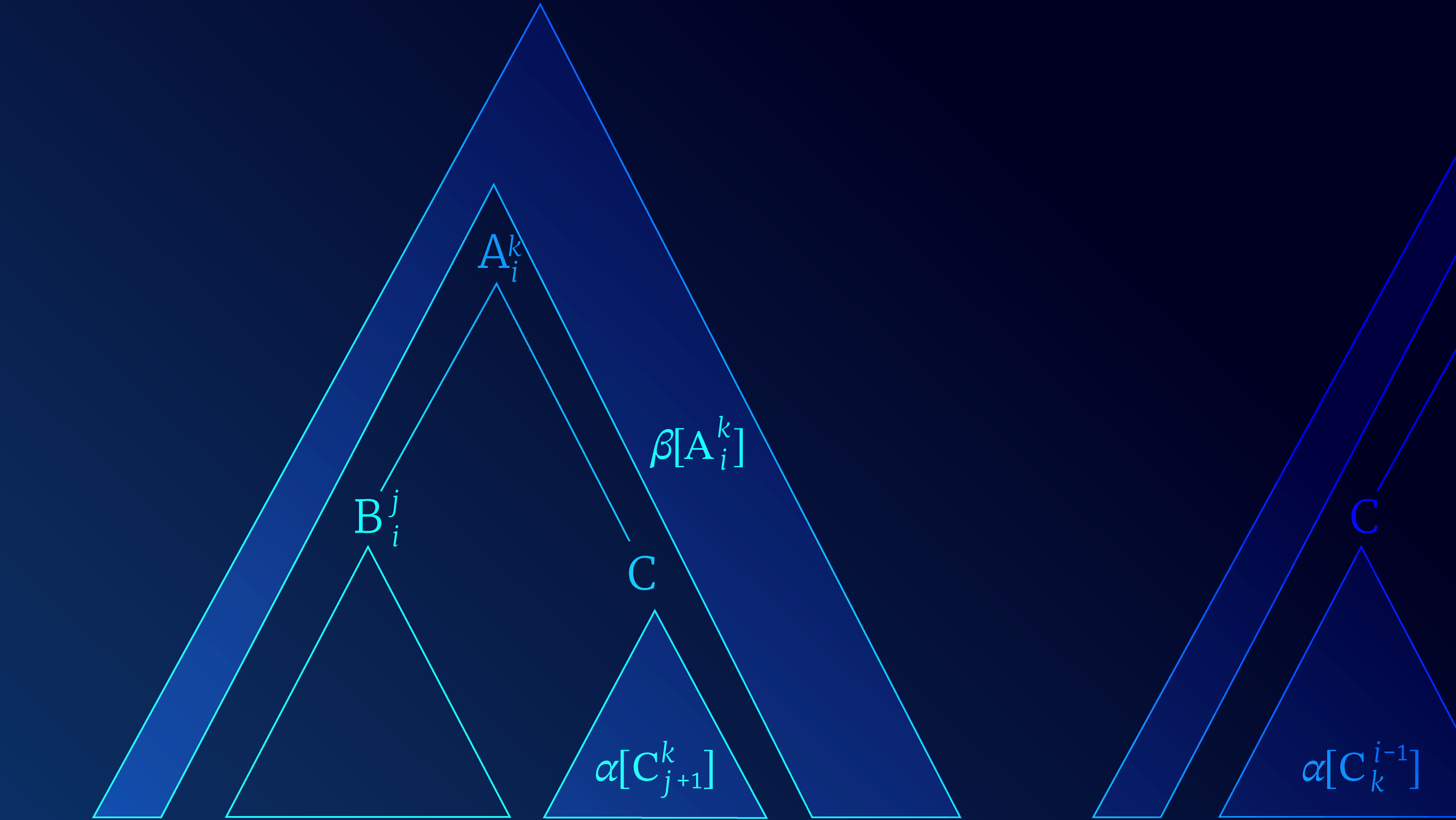
Figure 2. Outside weights. The outside weights $\beta[A_{i}^{k}$ consist of the sum of all the possible trees above and around $A_{i}^{k}$. We show the recursive update for $\beta[\text{B}_{i}^{j}]$ which is the outer weight of its parent A plus the inner weights of its sibling B, taking into account whether B is the first child (left) or second child (right), all possible values of A and C, and the split point $k$.
\begin{eqnarray} \beta[\text{B}_i^j] = & \sum_{\text{A}, \text{C}} \sum_{k=j+1}^{n} \mbox{g}[\text{A} \rightarrow \text{B} \text{C}] \times \alpha[\text{C}_{j+1}^{k}] \times \beta[\text{A}_i^k]\nonumber \\ &+\sum_{\text{A}, \text{C}} \sum_{k=0}^{i-1} \mbox{g}[\text{A} \rightarrow \text{C} \text{B}] \times \alpha[\text{C}_{k}^{i-1}] \times \beta[\text{A}_{k-1}^j] \tag{36}\end{eqnarray}
The outside-trees of $\text{A}_i^j$ are are the set of trees that are rooted in $S$ and yield $w_1, \ldots, w_{i-1}, \text{A}, w_{j+1} \ldots, w_n$, where $n$ is the sentence length. These are the trees that originate from $S$ and occur around $\text{A}_i^j$ (figure 2). The recursive update computes the outer weight in terms of the parent outer weight and the sibling inner weight. It sums over all possible parents, siblings, the order of the siblings (there is one term for each in the equation) and the split point $k$.
Combining inside and outside weights
We have seen that the inside weights sum over all inside-trees and the outside weights sum over all outside trees. It follows that total weight of all the parses that contain the anchored non-terminal $\text{A}_i^k$ is simply $\alpha[\text{A}_i^k] \cdot \beta[\text{A}_i^k]$. If we normalize by the partion function, $Z$ we retrieve the marginal probability of the anchored non-terminal $\text{A}_i^k$ which is given by $(\alpha[\text{A}_i^k] \cdot \beta[\text{A}_i^k)]/Z$.
By combining equations 30 and 34, we see how the inside- and outside-weights fit together to compute the expected counts:
\begin{equation} \mathbb{E}_{T}\left[\text{A} \rightarrow \text{B} \text{C}\right]= \frac{1}{Z} \times \sum_{1 \leq i \leq j \leq k \leq n} \mbox{g}[\text{A} \rightarrow \text{B} \text{C}] \times \beta[\text{A}_i^k] \times \alpha[\text{B}_i^j] \times \alpha[\text{C}_j^k] \tag{37}\end{equation}
This equation enumerates all possible spans, where A could be re-written to B and C (inside), but also considers every configuration that could happen around A.
Summary
In this blog, we introduced probabilistic context-free grammars and we discussed both supervised and unsupervised methods for learning their parameters. In the former case, we learn the rule weights from pairs of sentences and parse trees and there is a simple intuitive closed-form solution.
Then we considered the unsupervised case, where we only have access to the sentences. The first strategy we described is Viterbi training, which is fairly simple: we already know how to do weighted parsing to find the best trees for known parameters, and we also know how to maximize the likelihood of the parameters if we are given the trees. The Viterbi EM initializes the parameters randomly and then parses the entire corpus. Taking these parses as pseudo-labels, it re-estimates the parameters to maximize their likelihood. Then we iterate until convergence.
Viterbi training is sometimes called Viterbi EM, hard EM or self-EM. Variants include unsupervised parsing of different formalisms and methods to improve over vanilla supervised training. The same ideas have been adapted for image classification and segmentation.
We also discussed the soft-EM approach to unsupervised learning of rule weights in PCFGs. Rather than inferring the trees with the highest weight we computed the expected number of times each rule would appear in the parses. Then these expected counts were used to find the maximum likelihood estimates for the parameters. To compute these expected counts, we used the inside-outside algorithm, which can be summarized by the code snippet Z = inside(w, $\theta$); log(Z).backward(). Finally, we made a big leap and discussed how to mechanistically derive the outside-algorithm from the inside-pass to obtain the expected rule counts.
1 The Penn Tree Bank is not publicly available, but a free alternative is the QuestionBank which contains English questions annotated with trees.
Tutorial #18: Parsing II: WCFGs, the inside algorithm, and weighted parsing
News
Meet Turing by Borealis AI, an AI-powered text to SQL database interface
Blog
Tutorial #15: Parsing I context-free grammars and the CYK algorithm
Work with Us!
Impressed by the work of the team? Borealis AI is looking to hire for various roles across different teams. Visit our career page now and discover opportunities to join similar impactful projects!
Careers at Borealis AI