
Introduction
The current dominant paradigm in natural language processing is to build enormous language models based on the transformer architecture. Models such as GPT3 contain billions of parameters, which collectively describe joint statistics of spans of text and have been extremely successful over a wide range of tasks.
However, these models do not explicitly take advantage of the structure of language; native speakers understand that a sentence is syntactically valid, even if it is meaningless. Consider how Colorless green ideas sleep furiously feels like valid English, whereas Furiously sleep ideas green colorless does not 1. This structure is formally described by a grammar, which is a set of rules that can generate an infinite number of sentences, all of which sound right, even if they mean nothing.
In this blog, we review earlier work that models grammatical structure. We introduce the CYK algorithm which finds the underlying syntactic structure of sentences and forms the basis of many algorithms for linguistic analysis. The algorithms are elegant and interesting for their own sake. However, we also believe that this topic remains important in the age of large transformers. We hypothesize that the future of NLP will consist of merging flexible transformers with linguistically informed algorithms to achieve systematic and compositional generalization in language processing.
Overview
Our discussion will focus on context-free grammars or CFGs. These provide a mathematically precise framework in which sentences are constructed by recursively combining smaller phrases usually referred to as constituents.2 Sentences under a CFG are analyzed through a tree-structured derivation in which the sentence is recursively generated phrase by phrase (figure 1).

Figure 1. Parsing example for the sentence “The dog is in the garden.” The sentence is parsed into constituent part-of-speech (POS) categories represented in a tree structure. The POS categories and phrase types here are sentence (S), noun phrase (NP), determiner (DT), verb phrase (VP), present tense verb (VBZ), prepositional phrase (PP), preposition (P), and noun (NN).
The problem of recovering the underlying structure of a sentence is known as parsing. Unfortunately, natural language is ambiguous and so there may not be a single possible meaning; consider the sentence I saw him with the binoculars. Here, it is unclear whether the subject or the object of the sentence holds the binoculars (figure 2). To cope with this ambiguity, we will need weighted and probabilistic extensions to the context free grammar (referred to as WCFGs and PCFGs respectively). These allow us to compute a number that indicates how “good” each possible interpretation of a sentence is.

Figure 2. Parsing the sentence “I saw him with binoculars” into constituent part-of-speech (POS) categories (e.g. noun) and phrase types (e.g., verb phrase) represented in a tree structure. The POS categories and phrase types here are sentence (S), noun phrase (NP), verb phrase (VP), past tense verb (VBD), prepositional phrase (PP), preposition (P), determiner (DT), and noun (NN). a) In this parse, it is “I” who have the binoculars. b) A second possible parse of the same sentence, in which it is “him” who possesses the binoculars.
In Part I of this series of two blogs, we introduce the notion of a context-free grammar and consider how to parse sentences using this grammar. We then describe the CYK recognition algorithm which identifies whether the sentence can be parsed under a given grammar. In Part II, we introduce the aforementioned weighted context-free grammars and show how the CYK algorithm can be adapted to compute different quanties including the most likely sentence structure. In Part III we instroduce probabilistic context-free grammars, and we present the inside-outside algorithm which efficiently computes the expected counts of the rules in the grammar for all possible analyses of a sentence. These expected counts are used in the E-Step of an expectation-maximization procedure for learning the rule weights.
Parse trees
Before tackling these problems, we’ll first discuss the properties of a parse tree (figure 3). The root of the tree is labelled as “sentence” or “start”. The leaves or terminals of the tree contain the words of the sentence. The parents of these leaves are called pre-terminals and contain the part-of-speech (POS) categories of the words (e.g., verb, noun, adjective, preposition). Words are considered to be from the same category if a sentence is still syntactically valid when they are substituted. For example: The {sad, happy, excited, bored} person in the coffee shop. This is known as the substitution test. Above the pre-terminals, the word categories are collected together into phrases.
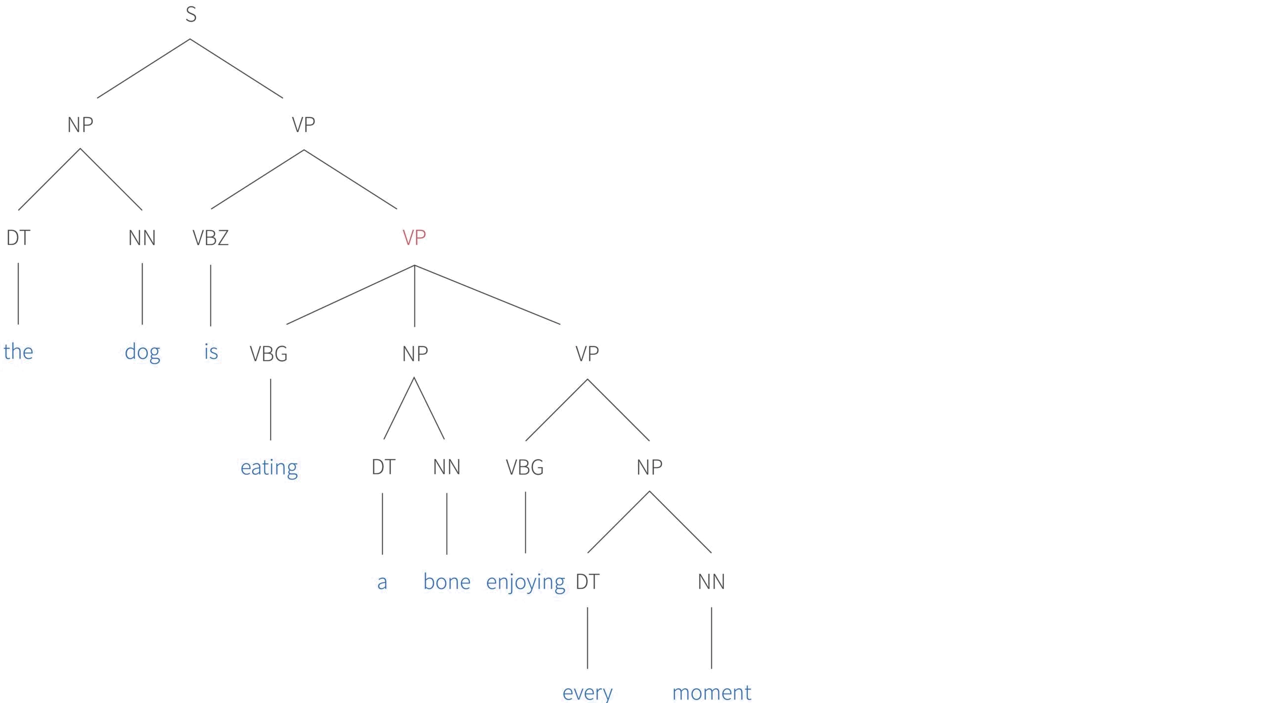
Figure 3. Parse tree for a more complex sentence. The POS categories here are sentence (S), noun phrase (NP), determiner (DT), noun (NN), verb phrase (VP), third person singular verb (VBZ), and gerund (VBG).
There are three more important things to notice. First, the verb phrase highlighted in magenta has three children. However, there is no theoretical limit to this number. We could easily add the prepositional phrases in the garden and under a tree and so on. The complexity of the sentence is limited in practice by human memory and not by the grammar itself.
Second, the grammatical structure allows for recursion. In this example, a verb phrase is embedded within a second verb phrase, which itself is embedded in a third verb phrase. Finally, we note that the parse tree disambiguates the meaning of the sentence. From a grammatical point of view, it could be that it was the bone that was enjoying every moment. However, it is clear that this is not the case, since the verb phrase corresponding to enjoying is attached to the verb phrase corresponding to eating and not the bone (see also figure 2).
Context free grammars
In this section, we present a more formal treatment of context-free grammars. In the following section, we’ll elucidate the main ideas with an example.
A language is a set of strings. Each string is a sequence of terminal symbols. In figure 3 these correspond to individual words, but more generally they may be abstract tokens. The set of terminals $\Sigma=\{\mbox{a,b,c},\ldots\}$ is called an alphabet or lexicon. There is also a set $\mathcal{V}=\{\mbox{A,B,C}\ldots…\}$ of non-terminals, one of which is the special start symbol $S$.
Finally, there are a set $\mathcal{R}$ of production or re-write rules. These relate the non-terminal symbols to each other and to the terminals. Formally, these grammar rules are a subset of the finite relation $\mathcal{R}\in \mathcal{V} \times (\Sigma \cup \mathcal{V})^*$ where $*$ denotes the Kleene star. Informally, this means that each grammar rule is an ordered pair where the first element is a non-terminal from $\mathcal{V}$ and the second is any possible string containing terminals from $\Sigma$ and non-terminal from $\mathcal{V}$. For example, B$\rightarrow$ab, C$\rightarrow$Baa and A$\rightarrow$AbCa are all production rules.
A context free grammar is the tuple $G=\{\mathcal{V}, \Sigma, \mathcal{R}, S\}$ consisting of the non-terminals $\mathcal{V}$, terminals $\Sigma$, production rules $\mathcal{R}$, and start symbol $S$. The associated context-free language consists of all possible strings of terminals that are derivable from the grammar.
Informally, the term context-free means that each production rule starts with a single non-terminal symbol. Context-free grammars are part of the Chomsky hierarchy of languages which contains (in order of increasing expressiveness) regular, context-free, context-sensitive, and recursively enumerable grammars. Each differs in the family of production rules that are permitted and the complexity of the associated parsing algorithms (table 1). As we shall see, context-free languages can be parsed in $O(n^{3})$ time where $n$ is the number of observed terminals. Parsing more expressive grammars in the Chomsky hierarchy has exponential complexity. In fact, context-free grammars are not considered to be expressive enough to model real languages. Many other types of grammar have been invented that are both more expressive and parseable in polynomial time, but these are beyond the scope of this post.
| Language | Recognizer | Parsing Complexity |
| Recursively enumerable Context-sensitive Context-free Regular | Turing machine Linear-bounded automata Pushdown automata Finite-state automata | decideable PSPACE $O(n^3)$ $O(n)$ |
Table 1. The Chomsky hierarchy of languages. As the grammar-type becomes simpler, the required computation model (recognizer) becomes less general and the parsing complexity decreases.
Example
Consider the context free grammar that generated the example in figure 4. Here, the set of non-terminals $\mathcal{V}=\{\mbox{VP, PP, NP, DT, NN, VBZ, IN,}\ldots\}$ contains the start symbol, phrases, and pre-terminals. The set of terminals $\Sigma=\{$The, dog, is, in, the, garden, $\ldots \}$ contains the words. The production rules in the grammar associated with this example include:

Of course, a full model of English grammar contains many more non-terminals, terminals, and rules than we observed in this single example. The main point is that the tree structure in figure 4 can be created by the repeated application of a finite set of rules.

Figure 4. Example sentence to demonstrate context free grammar rules
Chomsky Normal Form
Later on, we will describe the CYK recognition algorithm. This takes a sentence and a context-free grammar and determines whether there is a valid parse tree that can explain the sentence in terms of the production rules of the CFG. However, the CYK algorithm assumes that the context free grammar is in Chomsky Normal Form (CNF). A grammar is in CNF if it only contains the following types of rules:
\begin{align} \tag{binary non-terminal}
\text{A} &\rightarrow \text{B} \; \text{C} \\
\tag{unary terminal}
\text{A} &\rightarrow \text{a} \\
\tag{delete sentence}
\text{S} &\rightarrow \epsilon
\end{align}
where A,B, and C are non-terminals, a is a token, S is the start symbol and $\epsilon$ represents the empty string.
The binary non-terminal rule means that a non-terminal can create exactly two other non-terminals. An example is the rule $S \rightarrow \text{NP} \; \text{VP}$ in figure 4. The unary terminal rule means that a non-terminal can create a single terminal. The rule $\text{NN} \rightarrow$ $\text{dog}$ in figure 4 is an example. The delete sentence rule allows the grammar to create empty strings, but in practice we avoid $\epsilon$-productions.
Notice that the parse tree in figure 3 is not in Chomsky Normal Form because it contains the rule $\text{VP} \rightarrow \text{VBG} \; \text{NP} \; \text{VP}$. For the case of natural language processing, there are two main tasks to convert a grammar to CNF:
- We deal with rules that produce more than two non-terminals by creating new intermediate non-terminals (figure 5a).
- We remove unary rules like A →→ B by creating a new node A_B (figure 5b).

Figure 5. Conversion to Chomsky Normal form. a) Converting non-binary rules by introducing new non-terminal B_C. b) Eliminating unary rules by creating new non-terminal A_B.
Both of these operations introduce new non-terminals into the grammar. Indeed, in the former case, we may introduce different numbers of new non-terminals depending on which children we choose combine. It can be shown that in the worst-case scenario, converting CFGs into an equivalent grammar in Chomsky Normal Form results in a quadratic increase in the number of rules. Note also that although the CNF transformation is the most popular, it is not the only, or even the most efficient option.
Parsing
Given a grammar in Chomsky Normal Form, we can turn our attention to parsing a sentence. The parsing algorithm will return a valid parse tree like the one in figure 6 if the sentence has a valid analysis, or indicate that there is no such valid parse tree.

Figure 6. Example parse tree for the sentence Jeff trains geometry students. This sentence has $n=4$ terminals. It has $n-1=3$ internal nodes representing the non-terminals and a $n=4$ pre-terminal nodes.
It follows that one way to characterize a parsing algorithm is that it searches over the set of all possible parse trees. A naive approach might be to exhaustively search through these trees until we find one that obeys all of the rules in the grammar and yields the sentence. In the next section, we’ll consider the size of this search space, find that it is very large, and draw the conclusion that this brute-force approach is intractable.
Number of parse trees
The parse tree of a sentence of length $n$ consists of a binary tree with $n-1$ internal nodes, plus another $n$ nodes connecting the pre-terminals to the terminals. The number of binary trees with $n$ internal nodes can be calculated via the recursion:
\begin{equation}C_{n} = \sum_{i=0}^{n-1}C_{n-i}C_{i}. \tag{1}\end{equation}

Figure 7. Intuition for number $C_{n}$ of binary trees with $n$ internal nodes. a) There is only one tree with a single internal node, so $C_{1}=1$. b) To generate all the possible trees with $n=2$ internal nodes, we add a new root (red sub-tree). We then add the tree with $n=1$ node either to the left or to the right branch of this sub-tree to create the $C_{2} = C_{1}+C_{1} =2$ possible combinations. c) To generate all the possible trees with $n=3$ nodes, we again add a new root (green sub-tree). We can then add either of the trees with $n=2$ to the left node of this sub-tree, or d) add the tree with $n=1$ nodes to both the left and right, or e) add either of the trees with $n=2$ to the right node of this sub-tree. This gives a total of $C_{3} = C_{2} + C_{1}C_{1}+ C_{2} = 5$ possible trees. We could continue in this way and by the same logic $C_{4} = C_{3}+C_{2}C_{1}+C_{1}C_{2}+C_{3} = 14$. Defining $C_{0}=1$ we have the general recursion $C_{n} = \sum_{i=0}^{n-1}C_{n-i}C_{i}$.
The intuition for this recursion is illustrated in figure 7. This series of intergers are known as the Catalan number and can be written out explicitly as:
\begin{equation} C_n = \frac{(2n)!}{(n+1)!n!}. \tag{2}\end{equation}
Needless to say the series grows extremely fast:
\begin{equation} 1, 1, 2, 5, 14, 42, 132, 429, 1430, 4862, 16796, 58786, \ldots \tag{3}\end{equation}
Consider the example sentence I saw him with the binoculars. Here there are only C_5=42 possible trees, but these must be combined with the non-terminals in the grammar (figure 8). In this example, for each of the 42 trees, each of the six leaves must contain one of four possible parts of speech (DT, NN, P, VBD) and each of the five non-leaves must contain one of four possible clause types (S, NP, VP, PP) and so there are 42 * 4^6 * 4^5 = 176160768 possible parse trees.

Figure 8. Minimal set of grammar rules in Chomsky Normal Form for parsing example sentence I saw him with the binoculars. a) Rules relating pre-terminals to terminals. Note that the word saw is ambiguous and may be a verb (meaning observed) or as a noun (meaning a tool for cutting wood). b) Rules relating non-terminals to one another.
Even this minimal example had a very large number of possible explanations. Now consider that (i) the average sentence length written by Charles Dickens was 20 words, with an associated $C_{20}=6,564,120,420$ possible binary trees and (ii) that there are many more parts of speech and clause types in a realistic model of the English language. It’s clear that there are an enormous number of possible parses and it is not practical to employ exhaustive search to find the valid ones.
The CYK algorithm
The CYK algorithm (named after inventors John Cocke, Daniel Younger, and Tadao Kasami) was the first polynomial time parsing algorithm that could be applied to ambiguous CFGs (i.e., CFGs that allow multiple derivations for the same string). In its simplest form, the CYK algorithm solves the recognition problem; it determines whether a string $\mathbf{w}$ can be derived from a grammar $G$. In other words, the algorithm takes a sentence and a context-free grammar and returns TRUE if there is a valid parse tree or FALSE otherwise.
This algorithm sidesteps the need to try every possible tree by exploiting the fact that a complete sentence is made by combining sub-clauses, or equivalently, a parse tree is made by combining sub-trees. A tree is only valid if its sub-trees are also valid. The algorithm works from the bottom of the tree upwards, storing possible valid sub-trees as it goes and building larger sub-trees from these components without the need to re-calculate them. As such, CYK is a dynamic programming algorithm.
The CYK algorithm is just a few lines of pseudo-code:
0 # Initialize data structure
1  chart[1...n, 1...n, 1...V] := FALSE
2
3  # Use unary rules to find possible parts of speech at pre-terminals
4  for p := 1 to n   # start position
5    for each unary rule A -> w_p
6        chart[1, p, A] := TRUE
7
8  # Main parsing loop
9  for l := 2 to n   # sub-string length
10    for p := 1 to n-l+1     #start position
11        for s := 1 to l-1   # split width
12            for each binary rule A -> B C
13                chart[l, p, A] = chart[l, p, A] OR
                                     (chart[s, p, B] AND chart[l-s,p+s C])
14
15  return chart[n, 1, S]
The algorithm is simple, but is hard to understand from the code alone. In the next section, we will present a worked example which makes this much easier to comprehend. Before we do that though, let’s make some high level observations. The algorithm consists of four sections:
- Chart: On line 1, we initialize a data structure, which is usually known as a chart in the context of parsing. This can be thought of as an $ntimes n$ table where $n$ is the sentence length. At each position, we have a length $V$ binary vector where $V=|mathcal{V}|$ is the number of non-terminals (i.e., the total number of clause types and parts of speech).
- Parts of speech: In lines 4-6, we run through each word in the sentence and identify whether each part of speech (noun, verb, etc.) is compatible.
- Main loop: In lines 8-13, we run through three loops and assign non-terminals to the chart. This groups the words into possible valid sub-phrases.
- Return value: In line 15 we return TRUE if the start symbol $S$ is TRUE at position $(n,1)$.
The complexity of the algorithm is easy to discern. Lines 9-13 contain three for loops depending on the sentence length $n$ (lines 9-11) and one more depending on the number of grammar rules $|R|$ (line 12). This gives us a complexity of $\mathcal{O}(n^3 \cdot |R|)$.
To make the CYK algorithm easier to understand, we’ll use the worked example of parsing the sentence I saw him with the binoculars. We already saw in figure 2 that this sentence has two possible meanings. We’ll assume the minimal grammar from figure 8 that is sufficient to parse the sentence. In the next four subsections we’ll consider the four parts of the algorithm in turn.
Chart
Figure 9 shows the chart for our example sentence, which is itself shown in an extra row under the chart. Each element in the chart corresponds to a sub-string of the sentence. The first index of the chart $l$ represents the length of that sub-string and the second index $p$ is the starting position. So, the element of the chart at position (4,2) represents the sub-string that is length four and starts at word two which is saw him with the. We do not use the upper triangular portion of the chart.
The CYK algorithm runs through each of the elements of the chart, starting with strings of length 1 and working through each position and then moving to strings of length 2, and so on, until we finally consider the whole sentence. This explains the loops in lines 9 and 10. The third loop considers possible binary splits of the strings and is indexed by $s$. For position (4,2), the string can be split into saw $|$ him with the ($s=1$, blue boxes), saw him $|$ with the ($s=2$, green boxes), or saw him with $|$ the ($s=3$, red boxes).

Figure 9. Chart construction for CYK algorithm. The original sentence is below the chart. Each element of the chart corresponds to a sub-string so that position (l, p) is the sub-string that starts at position $p$ and has length $l$. For the $l^{th}$ row of the chart, there are $l-1$ ways of dividing the sub-string into two parts. For example, the string in the gray box at position (4,2) can be split in 4-1 =3 ways that correspond to the blue, green and red shaded boxes and these splits are indexed by the variable $s$.
Parts of speech
Now that we understand the meaning of the chart and how it is indexed, let’s run through the algorithm step by step. First we deal with strings of length $l=1$ (i.e., the individual words). We run through each unary rule $A \rightarrow w_p$ in the grammar and set these elements to TRUE in the chart (figure 10). There is only one ambiguity here, which is the word saw which could be a past tense verb or a noun. This process corresponds to lines 5-6 of the algorithm.

Figure 10. Applying unary rules in CYK algorithm. We consider the sub-strings of length 1 (i.e., the individual words) and note which parts of speech could account for that word. In this limited grammar there is only one ambiguity which is the word saw which could be the past tense of see or a woodworking tool. Note that this is the same chart as in figure 9 but the rows have been staggered to make it easier to draw subsequent steps in the algorithm.
Main loop
In the main loop, we consider sub-strings of increasing length starting with pairs of words and working up to the full length of the sentence. For each sub-string, we determine if there is a rule of the form $\text{A}\rightarrow \text{B}\;\text{C}$ that can derive it.
We start with strings of length $l=2$. These can obviously only be split in one way. For each position, we note in the chart all the non-terminals A that can be expanded to generate the parts of speech B and C in the boxes corresponding to the individual words (figure 11).

Figure 11. Main loop for strings of length $l=2$. We consider each pair of words in turn (i.e, work across the row $l=2$). There is only one way to split a pair of words, and so for each position, we just consider whether each grammar rule can explain the parts of speech in the boxes in row $l=1$ that correspond to the individual words. So, position (2,1) is left empty as there is no rule of the form $\text{A}\rightarrow \text{NP}\;\text{NN}$ or $\text{A}\rightarrow \text{NP}\;\text{VBD}$. Position (2,2) contains $\text{VP}$ as we can use the rule $\text{VP}\rightarrow \text{VBD}\:\text{NP}$ and so on.
In the next outer loop, we consider sub-strings of length $l=3$ (figure 12). For each position, we search for a rule that can derive the three words. However, now we must also consider two possible ways to split the length 3 sub-string. For example, for position $(3,2)$ we attempt to derive the sub-string saw him with. This can be split as saw him $|$ with corresponding to positions (2,2)$|$(1,4) which contain VP and P respectively. However, there is no rule of the form $\text{A}\rightarrow\text{VP}\;\text{P}$. Likewise, there is no rule that can derive the split saw $|$ him with since there was no rule that could derive him with. Consequently, we leave position $(3,2)$ empty. However, at position $(3,4)$, the rule $\text{PP}\rightarrow \text{P}\;\text{NP}$ can be applied as discussed in the legend of figure 12.

Figure 12. Main loop for strings $l=3$. We consider each triple of words in turn (i.e., work across the row $l=3$). We can split each triple in two possible ways and for each box we consider whether there is a rule that explains each split. For example, for position (3,4) corresponding to the sub-string with the binoculars, we can explain with by the non-terminal P from row $l=1$ and the binoculars with the non-terminal NP from row $l=2$ using the rule $\text{PP}\rightarrow\text{P}\;\text{NP}$. Hence, we add PP to position (3,4).
We continue this process, working upwards through the chart for longer and longer sub-strings (figure 13). For each sub-string length, we consider each position and each possible split and add non-terminals to the chart where we find an applicable rule. We note that position $(5,2)$ in figure 13b corresponding to the sub-string saw him with the binoculars is particularly interesting. Here there are two possible rules $\text{VP}\rightarrow\text{VP}\;\text{PP}$ and $\text{VP}\rightarrow\text{VBD}\;\text{NP}$ that both come to the conclusion that the sub-string can be derived by the non-terminal VP. This corresponds to the original ambiguity in the sentence.

Figure 13. Continuing CYK main loop for strings of a) length $l=4$ b) length $l=5$ and c) length $l=6$. Note the ambiguity in panel (b) where there are two possible routes to assign the non-terminal VP to position (5,2) corresponding to the sub-strings saw $|$ him with the binoculars and saw him $|$ with the binoculars. This reflects the ambiguity in the sentence ; it may be either I or him who has the binoculars.
When we reach the top-most row of the chart ($l=6$), we are considering the whole sentence. At this point, we discover if the start symbol $S$ can be used to derive the entire string. If there is such a rule, the sentence is valid under the grammar and if there isn’t then it is not. This corresponds to the final line of the CYK algorithm pseudocode. For this example, we use the rule $S\rightarrow \text{NP}\;\text{VP}$ explain the entire sting with the noun phrase I and the verb phrase saw him with the binoculars and conclude that the sentence is valid under this context free grammar.
Retrieving solutions
The basic CYK algorithm just returns a binary variable indicating whether the sentence can be parsed or not under a grammar $G$. Often we are interested in retrieving the parse tree(s). Figure 14 superimposes the paths that led to the start symbol in the top left from figures 11-13. These paths form a shared parse forest; two trees share the black paths, but the red paths are only in the first tree and the blue paths are only in the second tree. These two trees correspond to the two possible meanings of the sentence (figure 15).

Figure 14. Superimposition of paths that lead to the start symbol at position (6,1) from figures 11-13. These describe two overlapping trees forming a shared parse forest: the common parts are drawn in black, paths in only the first tree are in red and paths only in the second tree are only in blue. These are the parse trees for two possible meanings of this sentence.
These two figures show that it is trivial to reconstruct the parse tree once we have run the CYK algorithm as long as we cache the inputs to each position in the chart. We simply start from the start symbol at position (6,1) and work back down through the tree. At any point where there are two inputs into a cell, there is an ambiguity and we must enumerate all combinations of these ambiguities to find all the valid parses. This technique is similar to other dynamic programming problems (e.g.: the canonical implementation of the longest common subsequence algorithm computes only the size of the subsequence, but backpointers allow for retrieving the subsequence itself).

Figure 15. The two trees from figure 14 correspond exactly with the two possible parse trees that explain this sentence under the provided grammar. a) In this analysis, it is I who have the binoculars. b) A second possible analysis of the same sentence, in which it is him who has the binoculars.
A more challenging example
The previous example was relatively unambiguous. For a bit of fun, we’ll also show the results on the famously difficult-to-understand sentence Buffalo buffalo Buffalo buffalo buffalo buffalo Buffalo buffalo. Surprisingly, this is a valid English sentence. To comprehend it, you need to know that (i) buffalo is a plural noun describing animals that are also known as bison, (ii) Buffalo is a city, and (iii) buffalo is a verb that means “to indimidate”. The meaning of the sentence is thus:
Bison from the city Buffalo that are intimidated by other bison from the city Buffalo, themselves intimidate yet other bison from the city Buffalo.
To make things even harder, we’ll assume that the text is written in all lower case, and so each instance of buffalo could correspond to any of the three meanings. Could you come up with a grammar that assigns an intuitive analysis to this sentence? In Figure 16 we provide a minimal, but sufficient grammar that allows the CYK algorithm to find a single and reasonable parse tree for this strange sentence.

Figure 16. Running the CYK algorithm on the sentence buffalo buffalo buffalo buffalo buffalo buffalo buffalo buffalo. The CYK algorithm returns TRUE as it is able to put the start symbol $S$ in the top-left corner of the chart. The red lines show the tracing back of the parse tree to the constituent parts of speech.
CYK algorithm summary
In this part of the blog, we have described the CYK algorithm for the recognition problem; the algorithm determines whether a string can be generated by a given grammar. It is a classic example of a dynamic programming algorithm that explores an exponential search space in polynomial time by storing intermediate results. Another way of thinking about the CYK algorithm from a less procedural and more declarative perspective is that it is performing logical deduction. The axioms are the grammar rules and we are presented with facts which are the words. For a given sub-string length, we deduce new facts applying the rules of the grammar $G$ and facts (or axioms) that we had previous deduced about shorter sub-strings. We keep applying the rules to reach new facts about which sub-string is derivable by $G$ with the goal of proving that $S$ derives the sentence.
Note that we have used an unconventional indexing for the chart in our description. For a more typical presentation, consult these slides.
In part II, we will consider assigning probabilities to the production rules, so when the parse is ambiguous, we can assign probabilities to the different meanings. We will also consider the inside-outside algorithm which helps learn these probabilities.
1 This famous example was used in Syntactic Structures by Noam Chomsky in 1957 to motivate the independence of syntax and semantics.
2 The idea that sentences are recursively built up from smaller coherent parts dates back at least to a Sanskrit sutra of around 4000 verses known as Aṣṭādhyāyī written by Pāṇini probably around the 6th-4th century BC.
Tutorial #18: Parsing II: WCFGs, the inside algorithm, and weighted parsing
News
Meet Turing by Borealis AI, an AI-powered text to SQL database interface
Work with Us!
Impressed by the work of the team? Borealis AI is looking to hire for various roles across different teams. Visit our career page now and discover opportunities to join similar impactful projects!
Careers at Borealis AI