In this post we look at machine learning model debugging from a data centric perspective. After detecting a failure in a model, two important questions must be answered: 1) what is the reason of the failure? We follow a data centric approach and relate the failures to problematic training data points; and 2) how can we modify the model to mitigate the failure? To answer this question we introduce PUMA, a model patching algorithm that reduces the influence of the problematic training data points on the model parameters.
We first review some of the state of the art data valuation algorithms, which can be used to answer the first question and relate the issues in different model performance metrics to the training examples. In the second part, we review some of the state of the art model unlearning algorithms. These algorithms could be used to unlearn/remove the influence of the problematic training examples. However, as we will see, none of these algorithms can be used as a post-hoc modification algorithm and are mostly limited to the training objective. At the end, we introduce PUMA, our novel model patching algorithm that addresses the shortcomings of the available algorithms. PUMA reduces the negative impact of the problematic training examples on the model parameters, without re-training, while preserving its performance.
Model explanation & Model debugging
With recent successful applications of machine learning models in critical applications, such as healthcare and banking, the importance of model interpretability has become an important research topic. It is important and necessary to understand how the models make the decisions and to make sure these decisions are aligned with the business or legal regulations. Moreover, in the case of a failure, it is essential to understand the reason of the failure. There exist many algorithms that provide different insights about the model prediction process, using which we may find different issues in the model. However, they usually do not suggest a mitigation process for the discovered issues. Here, we propose a data centric model debugging process that helps the model developers and model validators in better understanding of the failures and to mitigate them.
In a data centric machine learning model debugging framework we should answer the following two questions: 1) can we use data valuation to find the training examples causing the model performance degradation? and 2) how can we modify the model parameters to remove the negative impact of the problematic training examples and to improve the performance of the model? Answering these two questions are the focus of this blog post.
To answer the first question, data valuation algorithms can be used [9, 10, 18, 19, 5]. Data centric mode interpretation algorithms are a class of algorithms that explain the model behavior by its training examples, e.g., by decomposing the model prediction into the influences of each training example on the prediction. In other words, data valuation algorithms relate the model performance to the training examples.
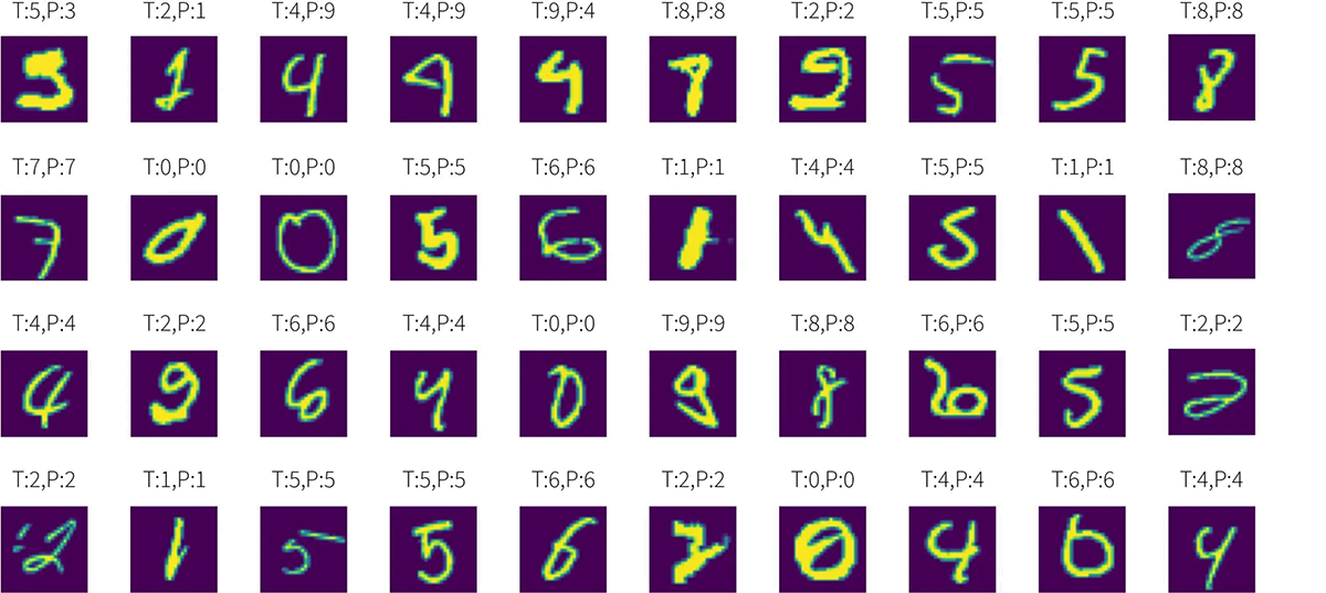
Figure 1: MNIST samples with confusing labels and images. Some of the images are even hard for ahuman to classify correctly. “T” shows the true label and “P” shows the model prediction.
To answer the second question, machine unlearning algorithms can be used to remove the negative effect of the detected problematic data points [6, 3, 15].
In the remainder of this post, we first review some papers that study the relation between the model failures and the issues in the training examples. We will continue with a brief review of the state of the art data valuation and unlearning algorithms. At the end, we introduce, PUMA, our novel model patching algorithm.
Data Quality and Model Performance
To motivate the rest of our discussion, in this section we first review papers that relate the quality of training data to model performance. The papers are mostly about the noisy labels, but we can extend it to the confusing labels as well, e.g., Imagenet samples with multiple targets in them and MNIST digits which resemble other digits (see figure 1) [16].
Quality of data and model performance
Generalization– generalization of deep learning has been studied in many literatures, from different perspectives, such as finding tight theoretical [7, 8] and numerical [7, 2] bounds for the generalization gap, and finding different approaches that improve the generalization of the models [14, 4]. Focusing on the papers that study the causes of large generalization gap, in [20, 1] it is shown that the effective capacity of neural networks is sufficient for memorizing the entire data set, even the noisy labels. This memorization severely affects the generalization of the models.
Calibration– Miscalibration is a mismatch between the prediction confidence score of the model and its correctness. This causes a mistrust in the predictions of the models, meaning that the confidence score could be over- or under-confident for different points. This is specially problematic for out of distribution generalization of the models, e.g., model could be wrong but very confident about its prediction. A potential cause of miscalibration is that Negative Log-Likelihood (NLL), commonly used in training classification models, is not a proper score as there is a gap between 0-1 accuracy and the loss measured by NLL [11]. A shortcut to reduce the NLL during training is to overfit to the easier examples to reduce the loss. As discussed in [11], this phenomena increases the miscalibration.
Adversarial Robustness– A connection between adversarial robustness and noisy labels is studied in [13]. Label noise is identified as one of the causes for adversarial vulnerability, and it provides theoretical and empirical evidences for this relation.
An emerging concept in above reviewed papers is the effect of the noisy labels and confusing training examples on the performance of the models, including robustness and generalization. This is mostly due to overfitting to the simpler examples. However, this is not always the case.
Fairness– Learning easier concepts faster and overfitting to the simple concepts in the training examples is studied in [12], as a cause of bias and unfairness in the model. Thus, in fairness, unlike the other reviewed cases, the issue is caused by learning and overfitting to the simpler concepts as a shortcut to make the predictions.
We use these studies as a motivation of our work in which we want to improve the model performance by removing the negative influence of the problematic data examples from the parameters of a trained model without re-training it.
Data Valuation
Now that we know the problematic training examples could affect the performance of a model, we will review some algorithms that help us to understand the effect of each training example on the model parameters and model predictions. We review these algorithms under the name of data valuation: the algorithms that assign an importance score showing the influence of each training example on a performance metric.
Data Shapley– Data Shapley, introduced in [5], is based on a method from coalitional game theory: a prediction can be explained by assuming that each training example is a “player” in a game where the model performance, e.g., accuracy, is the payout. Data Shapley values tells us how to fairly distribute the “payout” among the training data points. To calculate the exact Shapley values, a model should be trained for each combination of the presence of that example with other training examples to measure its performance
\begin{equation}
\phi_{i}=C \sum_{S \subseteq D-\{i\}} \frac{V(S \cup\{i\})-V(S)}{\left(\begin{array}{c}
n-1 \\
|S|
\end{array}\right)}
\end{equation}
We call φi the Data Shapley value of source i. The sum is over all subsets of training data D not containing training example i and C is an arbitrary constant. This computation is exponentially complex. Therefore, two estimate algorithms are proposed in [5]: Monte Carlo Shapely and Gradient Shapley. Gradient Shapley is only applicable in differentiable models while the Monte Carlo Shapley is more general and can be used for any model.
Reinforcement Learning based Data Valuation– A reinforcement learning based data valuation technique is proposed in [19], called DVRL. The main idea (shown in figure 2) is to learn a masking agent by REINFORCE algorithm [17] choosing the data examples that increase the performance of the model. The trained agent can be used as a data valuation model that assigns an importance score to each training data point. The major advantage of this algorithm is its applicability to any model even if the model is not differentiable.
Representer Point Selection (RPS)– RPS [18] decomposes the pre-activation predictions of a model into a linear combination of the pre-activation of its training data points. Denoting the pre-activation feature by Φ,fi= Φ (xi,Θ), and ˆyi= σ(Φ (xi,Θ)), where σ is the activation function and Θ is the model parameters, using RPS decomposition we have:
\begin{equation}
\Phi\left(\mathbf{x}_{t}, \Theta^{*}\right)=\sum_{i}^{n} k\left(\mathbf{x}_{t}, \mathbf{x}_{i}, \alpha_{i}\right)
\end{equation}
where $\alpha_{i}=\frac{1}{-2 \lambda n} \frac{\partial L\left(\mathbf{x}{i}, \mathbf{y}{i}, \boldsymbol{\Theta}\right)}{\partial \Phi\left(\mathbf{x}{i}, \boldsymbol{\Theta}\right)}$ ( $n$ is the number of training examples and $L$ is the loss function) and $k\left(\mathbf{x}{t}, \mathbf{x}{i}, \alpha{i}\right)=\alpha_{i} \mathbf{f}{i}^{T} \mathbf{f}{t} .$ The weights $\alpha_{i}$ of this linear combination can be used as a measure of the importance of the training examples in the model predictions. More accurately, these weights can be seen as the resistance for training example feature towards minimizing the norm of the weight matrix and therefore can be used to evaluate the importance of the training data points on the model
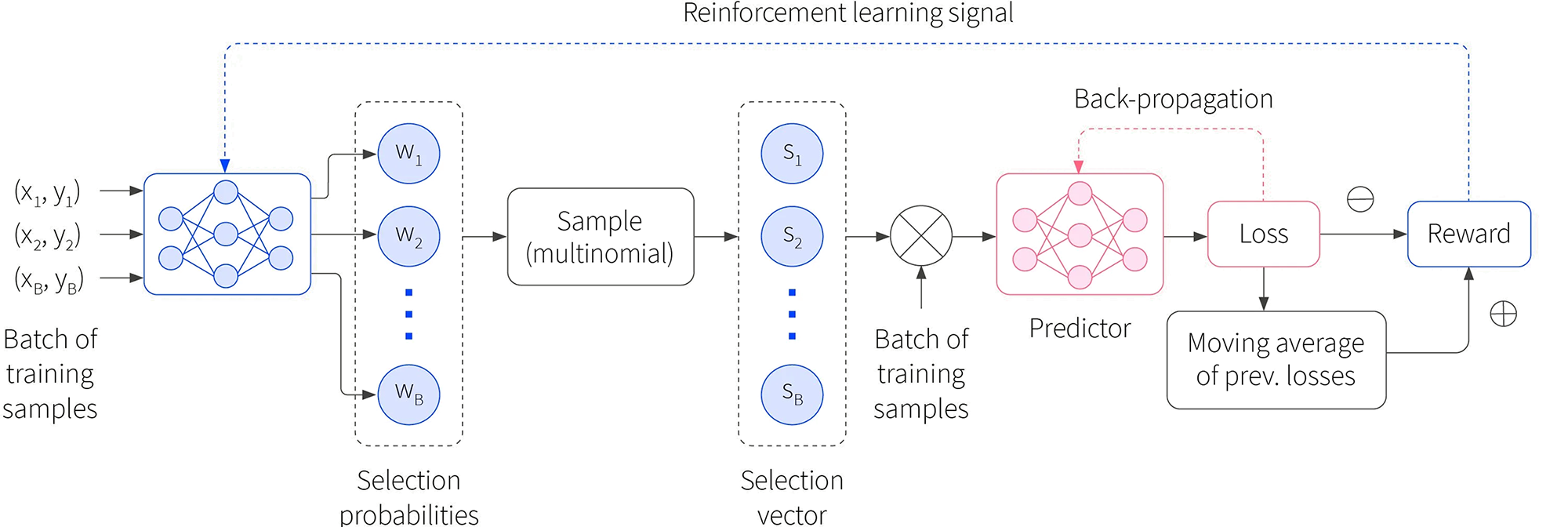
Figure 2: (Block diagram of the DVRL framework for training. A batch of training samples is usedas the input to the data value estimator (with shared parameters across the batch) and the output corresponds to selection probabilities of a multinomial distribution. The sampler, based on this multinomial distribution, returns the selection vector. The target task predictor model is trained only using the samples with selection vector, using gradient-descent optimization. (figure from [19]).
It should be noted that equation (2) holds only if the optimization objective of the model training has an ℓ2-norm weight decay of λ, and this algorithm is only applicable to differentiable neural networks.
Influence Functions– Influence functions is a classic technique from robust statistics to trace a model’s prediction through the learning algorithm and back to its training examples. Therefore, it could be used to identify the most responsible training examples for a given prediction. Influence functions require expensive second derivative calculations and assume model differentiability and convexity. In [10] efficient second-order optimization techniques are used to overcome some of the computation problems and used influence functions to explain deep neural networks.
The idea is to compute the parameter change if a sample z were upweighted by some smallε:
\begin{equation}
\hat{\theta}{\epsilon, z} \stackrel{\text { def }}{=} \arg \min_{\theta \in \Theta} \frac{1}{n} \sum_{i=1}^{n} L\left(z_{i}, \theta\right)+\epsilon L(z, \theta)
\end{equation}
The influence of this upweighting on the model parameters is given by:
\begin{equation}
\left.\mathcal{I}_{\text {up.params }}(z) \stackrel{\text { def }}{=} \frac{d \hat{\theta}_{\epsilon, z}}{d \epsilon}\right|_{\epsilon=0}=-H_{\hat{\theta}}^{-1} \nabla_{\theta} L(z, \hat{\theta})
\end{equation}
where $H_{\hat{\theta}} \stackrel{\text { def }}{=} \frac{1}{n} \sum_{i=1}^{n} \nabla_{\theta}^{2} L\left(z_{i}, \hat{\theta}\right)$ is the Hessian matrix. Using the chain rule we can calculate the influence of this upweighting on the loss function $L$, which can be used as the importance score of the training data examples:
$$
\begin{aligned}
\mathcal{I}_{\text {up }, \text { loss }}\left(z, z{\text {test }}\right) &\left.\stackrel{\text { def }}{=} \frac{d I_{\nu}\left(z_{\text {test }}, \hat{\theta}_{c, z}\right)}{d \epsilon}\right|_{\epsilon=0} ^{\mid}=\left.\nabla_{\theta} L\left(z_{\text {test }}, \hat{\theta}\right)^{\top} \frac{d \hat{\theta}_{\epsilon, z}}{d \epsilon}\right|_{\epsilon=0} \\
&=-\nabla_{\theta} L\left(z_{\text {test }}, \hat{\theta}\right)^{\top} H_{\hat{\theta}}^{-1} \nabla_{\theta} L(z, \hat{\theta})
\end{aligned}
$$
However, calculating the inverse Hessian is computationally very expensive. In [10] two estimation methods are suggested: 1) Conjugate gradients, and 2) stochastic estimation which uses Hessian vector product (HVP) to estimate the inverse Hessian.
Summary– The most important advantage of Data Shapley (specifically Monte Carlo Shapley) and DVRL compared to Influence functions and RPS is that we can use different performance measures other than the model loss objective. Influence functions and representer point selection explain the training data importance based on their contributions in the training loss objective. As a result, if we want to find the most influential training examples on fairness or calibration it cannot be done using RPS and Influence functions. In the next section you will see that our proposed algorithm, PUMA, modifies the Influence functions formulation and addresses this issue. Using PUMA’s modified formulation we can estimate the influence of the training examples on the model parameters in terms of different performance metric even if they are different from the training loss objective.
Unlearning and Model Patching
Up to here, we reviewed papers showing that some of the problems in model performance could be related to the problematic training examples. Then we reviewed data valuation algorithms that find the most influential training examples on the model parameters and the model performance.
Now, the question is if we can remove the negative influence of these problematic data points from the model parameters.
This concept is highly related tounlearning. In this section, we first review few papers focusing on unlearning some of the training examples from the model parameters.
SISA– To remove the influence of some specific training examples we may retrain a model after removing those examples. However, if a model and the training data points is large, the retraining could be computationally very expensive. In addition, beside the negative impacts, every data point has useful influence on the model parameters, which will be removed when re-training the model from scratch. Sharded, Isolated, Sliced, and Aggregated (SISA) [3] addresses the full re-training of a model by training sub-models on data shards and voting among the sub-model decisions to make the final decision. Using the data shards, we only need to re-train the sub-models that are affected by the removed data points.
Amnesiac Machine Learning (AML)– To remove the influence of the training data points from the learned parameters, [6] tracks the gradients of each data point (or batch of the data points) and removes the accumulated effect of the tracked gradients associated to the removed data points (or batches that data points are placed in) during the learning process from the model parameters. Since the gradient removing does not have a constraint to preserve the model performance after unlearning, the updated model is fine tuned for few epochs to recover the degraded performance.
Unrolling SGD (UrSGD)– Using the idea in Amnesiac Machine Learning, [15] removes the effect of the gradients from the model parameters. To improve the memory efficiency, instead of tracking the gradients during the training process a recursive gradient estimation is proposed using the first order gradients w.r.t the initial weights/parameters, and ignoring the higher level gradients. To improve this recursive estimation a regularizati term is proposed to be added to the training objective that minimizes the effect of the higher order gradients.
Summary– There is a limited number of studies available for model unlearning that could be used for our goal of removing negative impact of the problematic training data points. The available algorithms have one or more of the following shortcomings that makes them not suitable for our goal (figure 3):
- (SISA, AML) the training process is changed to accommodate the unlearning.
- (SISA, AML, UrSGD) there is no constraint on preserving the model performance duringthe modification process, and therefore the performance may degrade.
Performance Unchanged Model Augmentation (PUMA)
To estimate the influence of the training examples on the model parameters we follow influence functions derivation. Our goal is to modify the model parameters without seriously hurting its prediction performance with respect to various performance criteria C (or Lc for an individual sample) such that
\begin{equation}
\underbrace{\mid \frac{1}{\left|D_{t n}\right|} \sum_{i=1}^{\left|D_{t n}\right|} \mathcal{L}_{c}\left(\mathbf{x}_{i}, y_{i}, \theta_{m o d}\right)}_{\mathcal{C}\left(\theta_{m a d}\right)}-\underbrace{\frac{1}{\left|D_{t n}\right|} \sum_{i=1}^{\left|D_{t n}\right|} \mathcal{L}_{c}\left(\mathbf{x}_{i}, y_{i}, \theta_{o r g}\right)}_{\mathcal{C}\left(\theta_{o r g}\right)} \mid \leq \delta
\end{equation}
where $\delta>0$ is the performance drop limit, $\theta_{\text {mod }}$ is the modified model parameters, $\theta_{\text {org }}$ is the original model parameters, $\left|D_{\mathrm{tn}}\right|$ is the number of training data examples, and $\left(\mathbf{x}{i}, y{i}\right)$ is $i$-th training example and its corresponding target.

Figure 3: A scenario for model debugging and patching. Left: we run adversarial test and the model fails. Using data valuation we relate the issue to the training examples. Right: after modifying the model patching, the adversarial robustness test passes, but now the fairness test fails due to the new modifications.
Model modifications in PUMA is done by reweighting the training examples where the weights λ controls the contribution of each training example in the model modification:
\begin{equation}
\begin{aligned}
&\theta_{\bmod }=\underset{\theta}{\operatorname{argmin} \mathcal{J}_{\mathrm{mod}}(\theta)=} \\ &\underset{\theta}{\operatorname{argmin}} \underbrace{\frac{1}{\mid D_{\mathrm{tn} \mid}} \sum_{i=1}^{\left|D_{\mathrm{tn}}\right|} \mathcal{L}_{t}\left(\mathbf{x}_{i}, y_{i}, \theta\right)}_{\mathcal{J}_{\mathrm{org}}(\theta)}+\underbrace{\frac{1}{\left|D_{\mathrm{up}}\right|} \sum_{j=1}^{\left|D_{\mathrm{up}}\right|} \lambda_{j} \mathcal{L}_{t}\left(\mathbf{x}_{j}, y_{j}, \theta\right)}_{\mathcal{J}_{\mathrm{add}}(\theta)}
\end{aligned}
\end{equation}
where J is the training objective, Lt denotes individual prediction loss, Dup ⊆ Dtn is a subset of training examples used to compensate the effect of the removed examples.
Using this definition of the modified parameters and Taylor expansion of the gradient of $\mathcal{J}_{\bmod }(\theta)$ as the estimated update, we have:
$$
\begin{gathered}
\phi\left(\mathbf{x}_{i}, y_{i}\right)=\left(\nabla^{2} \mathcal{J}_{\text {org }}\left(\theta_{\text {org }}\right)\right)^{-1} \nabla \mathcal{L}_{t}\left(\mathbf{x}_{i}, y_{i}, \theta_{\text {org }}\right) \\
\theta_{\text {mod }}-\theta_{\text {org }}=-\sum_{j=1}^{\left|D_{\text {up }}\right|} \lambda_{j} \phi\left(\mathbf{x}_{j}, y_{j}\right)
\end{gathered}
$$
Now we can use this relation to estimate the changes in any performance metric C, which could be different from the training objective. Let’s introduce the following notation
\begin{equation}
\psi\left(\mathbf{x}{j}, y{j}\right)=\nabla \mathcal{C}\left(\theta_{\text {org }}\right)\left(\nabla^{2} \mathcal{J}{\text {org }}\left(\theta{\text {org }}\right)\right)^{-1} \nabla \mathcal{L}{t}\left(\mathbf{x}{j}, y_{j}, \theta_{\text {org }}\right)
\end{equation}
Data Valuation– ψ(xj,yj) can be used to valuate the importance of the training examples in the performance of the model, measured by C. Using this notation and Taylor expansion, we have the following estimation for the model performancechange after modifying its parameters:
\begin{equation}
\mathcal{C}\left(\theta_{\mathrm{mod}}\right)-\mathcal{C}\left(\theta_{\mathrm{org}}\right)=\nabla \mathcal{C}\left(\theta_{\mathrm{org}}\right)\left(\theta_{\mathrm{mod}}-\theta_{\mathrm{org}}\right)+\epsilon \approx-\sum_{j=1}^{\left|D_{\mathrm{up}}\right|} \lambda_{j} \psi\left(\mathbf{x}{j}, y{j}\right)
\end{equation}
The above equation enables us to not only estimate the effect of parameter modifications on the training objective, but also on any differentiable performance metric.

Figure 4: Projection Direction Comparison between Naive Influence Removal and PUMA. (a) The projection direction of each data point (black arrow as denoted byφ(xi,yi)). Blue arrow shows the one marked to remove. (b) The overall projection direction (red arrow) is toward high loss area after naive data contribution removal. (c) The overall projection direction (red arrow) is toward low loss area after PUMA data removal. Orange contour plot shows the loss surface of training objectiveJ. Purple contour plot shows the loss surface of performance criterion C. For both contour plots, lighter color shows lower loss.
Now we have the tools to get into the most important step of PUMA. To remove the negative effect of the problematic training examples from the model parameters the weight is set to λj=−1. To preserve the performance of the model as much as possible, PUMA compensates the influence ofthe removed training data examples by upweighting the influence of the remaining data points (or a subset of them). To do this upweighting optimally, we solve the following optimization problem to find the optimal weights:
\begin{equation}
\boldsymbol{\lambda}^{*}=\underset{\boldsymbol{\lambda}}{\operatorname{argmin}}\left\|\sum_{j \notin D_{\mathrm{mk}}}^{\left|D_{\mathrm{up}}\right|} \lambda_{j} \psi\left(\mathbf{x}_{j}, y_{j}\right)-\sum_{k=1}^{\left|D_{\mathrm{mk}}\right|} \psi\left(\mathbf{x}_{k}, y_{k}\right)\right\|^{2}+\Omega(\boldsymbol{\lambda})
\end{equation}
where $D_{m k}$ is the data points marked to be removed, $D_{\text {up }}$ is the subset of data to be upweighted, and $\Omega$ is a regularization term to sparsify the weights. Figure 4 depicts the importance of reweighting.
Model Patching – Knowing the optimal weights, we can use the following equation to update the model parameters:
$$
\theta_{\mathrm{mod}}=\theta_{\mathrm{org}}+\eta\left[\sum_{k=1}^{\left|D_{\mathrm{mk}}\right|} \phi\left(\mathbf{x}{k}, y{k}\right)-\sum_{j \notin D_{\mathrm{mk}}}^{\left|D_{\mathrm{up}}\right|} \lambda_{j}^{*} \phi\left(\mathbf{x}{j}, y{j}\right)\right]
$$
Summary–
- We can use ψ(xj,yj) to estimate the influence of the training examples in a performancemetric, which could be different from the training objective.
- To modify the model parameters:
- Select the data points to be removed: either as a prior knowledge or using a datavaluation algorithm.
- Estimate the inverse Hessian using methods suggested in [10].
- Find the optimal λ∗using equation (9).
- Use equation (10) to modify the model parameters.
Experiment
Here we present few experiment results showing the data valuation and model patching performance of PUMA. For extensive experiment results and comparisons with state of the art algorithms refer to the paper and its appendix.

Figure 5: Mislabelling debugging comparison between PUMA and state-of-the-art debugging algorithms. We corrupted datasets by randomly flipping 10% of the data labels. The goal of the candidate approaches is to identify and correct the mislabelled data as early as possible. PUMA shows significant advantage when only 20% of data are processed during debugging.

Figure 6: Removing the training points marked by crosses from the model. As demonstrated in the right plot, PUMA successfully removed the information of all marked points. `x’ in the plot shows the data intended to remove. Colors show the class labels.
Data Valuation– PUMA extends and generalizes the Influence functions, which is limited to the training objective, to incorporate different performance metrics. In PUMA’s formulation ψ(xj,yj) can be used as a data importance value. Figure 5 compares PUMA with some of the state of the art data valuation algorithms in detecting noisy labels. In this experiment we flip the labels of 10% of the training data points. The goal is to find the most number of noisy labels with least data investigation. We expect the data points with the lowest data value to be the ones with noisy labels. Therefore, we sort the data points according to their data values and investigate different portions of the data. As can be seen in figure 5 PUMA out performs others, or is at least as good as them. It should be noted that this is not the main goal of PUMA, but is a co-product of its formulation.
Model Patching: Data Removal– The main goal of PUMA is to remove the effect of the data points. To show PUMA’s success in removing the training points from model parameters, we present two examples here: using 1) a synthetic data (Radial dataset), and 2) MNIST.
In the first example, figure 6, we want to remove a cluster of the data points in the green class. The results show that those data points are successfully removed, without affecting the accuracy of the model in classifying the remaining data points in both classes.
In the second example we use MNIST dataset and aim to remove some of the images in class “4” with a specific style (the styles are clustered using K-means). As can be seen in figure 7, those “4”s are removed successfully (are classified as “6”) without affecting the other “4”s and other digits.
Model Patching: Calibration– We aim to improve the calibration of the model measured by Expected Calibration Error (ECE). ECE measures the gap between the average model confidence and its accuracy in bins of the model confidence.

Figure 7: Removing marked data points that belong to a particular style of digit 4. On top of eachdigit image, we show the ground truth label (denoted as T), predicted label (denoted as P), and theprediction confidence (denoted as Prob).

Figure 8: Problematic data points discovered by PUMA. The problems are categorized into three categories. For the prediction of mislabelled data points, we show the prediction’s True Positive (TP),False Positive (FP), and False Negative (FN).
In this example we use a two moon synthetic dataset, shown in figure 8 with 10% random label noise. First, PUMA’s data importance values are used to detect the training points that are more involved in increasing the miscalibration. Figure 8 shows three different types of detected data points: 1) data examples with noisy labels, 2) over-confident examples, and 3) under-confident examples. Then, PUMA is used to remove data points with noisy labels and a subset of the over-confident data points;and the under-confident points are up-weighted. The ECE improvement is obvious in figure 9 after augmenting the model parameters.

Figure 9: Expected Calibration Error (ECE) before and after PUMA model patching/augmentation.For most of prediction confidence bins, we observe the better calibration after PUMA model augmentation.
References
[1]Devansh Arpit et al. “A closer look at memorization in deep networks”. In:InternationalConference on Machine Learning. PMLR. 2017, pp. 233–242.
[2]Peter Bartlett, Dylan J Foster, and Matus Telgarsky. “Spectrally-normalized margin boundsfor neural networks”. In:arXiv preprint arXiv:1706.08498(2017).
[3] Lucas Bourtoule et al. “Machine unlearning”. In:arXiv preprint arXiv:1912.03817(2019).
[4]Pierre Foret et al. “Sharpness-aware minimization for efficiently improving generalization”. In:arXiv preprint arXiv:2010.01412(2020).
[5]Amirata Ghorbani and James Zou. “Data shapley: Equitable valuation of data for machinelearning”. In: International Conference on Machine Learning. PMLR. 2019, pp. 2242–2251.
[6]Laura Graves, Vineel Nagisetty, and Vijay Ganesh. “Amnesiac Machine Learning”. In: arXivpreprint arXiv:2010.10981(2020).
[7]Yiding Jiang et al. “Fantastic generalization measures and where to find them”. In: arXivpreprint arXiv:1912.02178(2019).
[8]Kenji Kawaguchi, Leslie Pack Kaelbling, and Yoshua Bengio. “Generalization in deep learn-ing”. In: arXiv preprint arXiv:1710.05468(2017).
[9]Been Kim, Rajiv Khanna, and Oluwasanmi O Koyejo. “Examples are not enough, learn to crit-icize! Criticism for Interpretability”. In: Advances in Neural Information Processing Systems.Ed. by D. Lee et al. Vol. 29. Curran Associates, Inc., 2016.URL:https://proceedings.neurips.cc/paper/2016/file/5680522b8e2bb01943234bce7bf84534-Paper.pdf.
[10]Pang Wei Koh and Percy Liang. “Understanding black-box predictions via influence functions”.In: International Conference on Machine Learning. PMLR. 2017, pp. 1885–1894.
[11]Jishnu Mukhoti et al. “Calibrating deep neural networks using focal loss”. In: arXiv preprintarXiv:2002.09437(2020).
[12]Junhyun Nam et al. “Learning from failure: Training debiased classifier from biased classifier”.In: arXiv preprint arXiv:2007.02561(2020).10
[13]Amartya Sanyal et al. “How benign is benign overfitting?” In: arXiv preprint arXiv:2007.04028(2020).
[14]David Stutz, Matthias Hein, and Bernt Schiele. “Relating adversarially robust generalization toflat minima”. In:Proceedings of the IEEE/CVF International Conference on Computer Vision.2021, pp. 7807–7817.
[15]Anvith Thudi et al. “Unrolling sgd: Understanding factors influencing machine unlearning”.In:arXiv preprint arXiv:2109.13398(2021).
[16]Sunil Thulasidasan et al. “Combating label noise in deep learning using abstention”. In: arXivpreprint arXiv:1905.10964(2019).
[17]Ronald J Williams. “Simple statistical gradient-following algorithms for connectionist rein-forcement learning”. In:Machine learning8.3 (1992), pp. 229–256.
[18]Chih-Kuan Yeh et al. “Representer point selection for explaining deep neural networks”. In:arXiv preprint arXiv:1811.09720(2018).
[19]Jinsung Yoon, Sercan Arik, and Tomas Pfister. “Data valuation using reinforcement learning”.In:International Conference on Machine Learning. PMLR. 2020, pp. 10842–10851.
[20]Chiyuan Zhang et al. “Understanding deep learning (still) requires rethinking generalization”.In:Communications of the ACM64.3 (2021), pp. 107–115.