Why is Cross-Domain Text-to-SQL Hard

Introduction

People communicate in natural language, which is flexible but often vague, whereas computer languages have no room for ambiguity. For a computer to respond to users’ questions or commands in natural language, it needs to extract meaning, resolve ambiguity, and translate to executable programs. This is the task of semantic parsing (SP), whose applications include voice assistants, code generation, natural language interfaces to databases (NLDB), and many more. Our Turing by Borealis AI system is an NLDB, a software system enabling users to interact with databases in natural language, as illustrated in Figure 1.

Figure 1. A natural language database interface (NLDB), like our turing system ($B$), translates a natural language question ($A$) to its corresponding SQL query ($C$), executes the query against the database ($D$), and finally returns the answer back to the user ($E$).

The semantic parsing model powering an NLDB needs to be trained with questions and their corresponding SQL queries. If the model only generalizes to new questions on the training domain, the NLDB cannot be quickly adapted to new databases, so it would not be very useful in practice. Hence, the model somehow needs to generalize to new databases with unseen schema and unseen questions. This is cross-domain or cross-database text-to-SQL semantic parsing.

The goal of this blog post is to glimpse into how models (like our Turing by Borealis AI system) for this task work without popping the hood. It is suitable for any reader with basic knowledge of machine learning and natural language processing.

We will first give a brief review of SQL that readers can skip if already familiar, then introduce two running examples of text-to-SQL prediction. The examples will illustrate some challenges involved in cross-domain semantic parsing and illustrate why simple methods would not succeed. Afterwards, we will describe a high-level framework that treats cross-database text-to-SQL as a graph-to-tree mapping. We will use the two running examples, to show how the framework tackles the challenges that we identified. Finally, we will provide some pointers for interested readers to learn more, including our recent ACL papers (Xu et al., 2021a,b; Norouzi et al., 2021) that respectively set the new state-of-the-art accuracy on the Spider text-to-SQL benchmark and some code generation problems.

SQL Primer

Before showing the examples, let us review some SQL basics. SQL stands for Structured Query Language and is used for storing, manipulating and retrieving data in relational databases. We will just focus on the retrieval here.

Relational databases store information records in tables. The schema of a database describes the structure of the domain: what are the tables, what columns does each table contain, the data type of each column, as well as special roles that some columns play. The first type of special role is a primary key. This is a column or a combination of columns that has to be unique for each data record. The second type of special role is a foreign key, which is a column or combination of columns whose values match the primary key records of another table. Foreign key relations link tables together.

Two text-to-SQL examples

To predict the correct SQL from a natural language question, the model needs to correctly interpret each input word in the context of both the sentence and the schema. Furthermore, it needs to generate a syntactically correct SQL query as the output otherwise the database cannot execute it. To illustrate the challenges more concretely, let’s consider two examples for the “Employee_hire_evaluation” database of the Spider benchmark. This database is a development set domain that models would not have seen during training.

SELECT employee.cityFROM employeeWHERE employee.age [COMP_A] [A]GROUP BY employee.cityHAVING COUNT (*) [COMP_C] [C]

Cross-database semantic parsing as graph-to-tree mapping

As shown by the two running examples, successful cross-database SQL semantic parsing really requires the model to reason using at least three sets of knowledge:

We now describe a general framework for cross-database text-to-SQL that leverages all of this knowledge. The backbone of the overall system is a neural network with encoder-decoder architecture, which is adapted in various ways to leverage explicit symbolic knowledge.

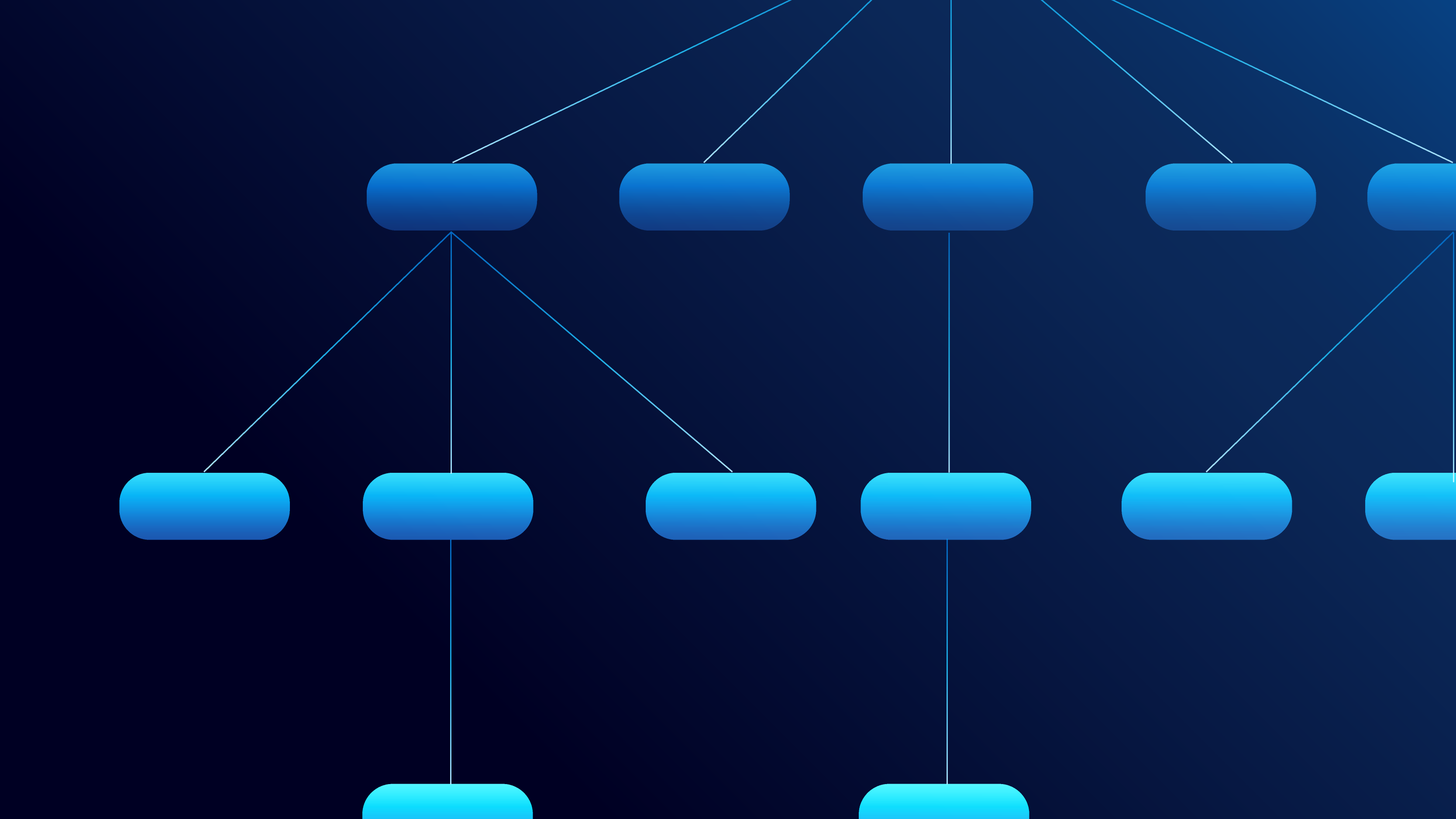
Figure 2. Overview of the graph-to-tree framework processing Example One. On the input side, the question and schema are modelled jointly as a graph. Between every pair of tokens within and across the question and schema, there is an implicit edge, which is not drawn for visual simplicity. Additionally, some edges carry special meanings, which are drawn with different colours. Some correspond to foreign key relations in the schema (in green) , while others correspond to lexicon evidence linking a question token to a schema element (red for exact word match; yellow for partial word match). On the output side, we model the SQL as its abstract syntax tree rather than a linear string. The tree structure embodies our prior knowledge of SQL grammar and its compositionality.

Motivated by the examples, we see that the model needs to jointly encode the question and schema, considering how words relate to each other within and across the question and the schema. So the input for cross-database semantic parsing has an inherent graph structure; the nodes are the tokens in the questions and schema and are linked by different edges. On the output side, to produce grammatically correct SQLs and leverage programming-language-specific inductive prior, we treat the prediction problem as generation of the abstract syntax tree (AST) of the program. Hence, we can characterize this task a graph-to-tree mapping.

Figure 2 illustrates the overall framework for Example One: an encoder consumes the input graph, and a decoder produces the output AST. Joint modelling of question and schema as a graph was popularized by the relation-aware transformer (RAT) work (Wang et al., 2019) while TranX (Yin and Neubig, 2018) provides a unified framework for modelling output programs as ASTs. Our Turing by Borealis AI system also follows this overall approach, with many additional innovations that we will not cover here.

Question-Schema joint encoding

As mentioned above, we view each token in the question and schema as a node in a graph. The most basic edge type among the nodes is a generic link between any pair of tokens, reflecting the assumption that a-priori any token could provide relevant context to any other token, so a link cannot be ruled out. This essentially yields a fully connected graph. For visual simplicity, we omit these edges from Figure 2.

However, other types of relations carry special meanings and are sparse. These include (i) foreign key relations that link a column in one table to the primary key of another table, (ii) exact string match and partial string match between words in the questions and words in column or table names and (iii) implicit links between a table and its columns. Some of these edges are illustrated in different colours on the input side in Figure 2. Because there can be more than one type of edge between two tokens to be modelled, this input is technically a multi-graph.

How do these edges help predict the correct SQL? Let’s return to the examples.

Example Two

The second example is more interesting. The question mentions the table name shop explicitly, while the table employee can be easily inferred based on the column mention age. However, for hiring there is no textual evidence from the question, direct or indirect, that the SQL query should involve hiring. The only way to infer is through the foreign key links and the fact that otherwise shop and employee are disconnected and cannot be joined. This potential reasoning process is illustrated in Figure 3.

Figure 3. Foreign key relations among tables help infer the missing information not present in the question. a) if the foreign key relationships of the schema are not modelled (hence in grey), there is no way to infer that table hiring is needed in this case. b) with the foreign key links modelled (in green), the structure of schema shows that hiring is the needed the missing link between employee and shop, even though there are no direct textual cues from the question.

Now that we understand how the (multi-)graph structure would help the semantic parsing model, let’s formalize what the encoder does at a high level. Let $\mathcal{S}=\{s_1,\dots, s_{\lvert \mathcal{S} \rvert}\}$ denote the schema elements, consisting of tables and their columns, and use $Q=q_1\dots q_{\lvert Q \rvert}$ to denote the sequence of words in the question. Let $\mathcal{G}=\langle\mathcal{V}, \mathcal{E}\rangle$ denote the multi-graph with edge sets $\mathcal{E}$. The encoder, $f_{\text{enc}}$, maps $\mathcal{G}$ to a joint representation $ \mathcal{H} =$ $\{\phi^q_1, \ldots,\phi^q_{\lvert Q \rvert} \} \cup \{\phi^s_1, \ldots,\phi^s_{\lvert \mathcal{S} \rvert} \}$. The fully connected portion of the multi-graph can be well modelled by a transformer (see [link] for our blog series on Transformers). Indeed, one can flatten the schema into a linear string, with the tokens belonging to different column or table names separated by a special token like “[SEP]” and concatenate this string with the question string before feeding into a pre-trained model such as BERT. The use of pre-trained BERT (or other variants) here is how implicit common sense knowledge is embodied in the semantic parser. To model information propagation along the special sparse edges of the multi-graph, we can then feed the BERT output embeddings into a relation-aware transformer (Wang et al., 2019). There are a few subtle details omitted here, which we will give some pointers for at the end of this article.

Grammar-based decoding

If we model SQL queries as linear sequences of text tokens on the output side, it is not easy to leverage the SQL grammar knowledge. During inference, one could use a grammar validator program to check if a generated sequence is legal; however, the neural network is still not using this information during training for better generalization. Furthermore, the grammar not only captures what is illegal but also how SQL expressions can be composed. Leveraging this prior knowledge will significantly improve the learning efficiency from a small number of examples. Therefore, we want to cast the problem as generating the abstract syntax tree of SQL queries.

Figure 4. How the TranX framework makes symbolic grammar knowledge accessible to a neural decoder: instead of directly predicting tokens of surface SQL code, the model would predict the sequence of AST-constructing action sequences. Before training, we preprocess the SQL code string by transforming it into its AST ($B$ $\leftarrow$ $C$). Then the TranX transition system builds the action sequences ($A$ $\leftarrow$ $B$) guided by the SQL grammar, expressed in the abstract syntax description language of TranX ($G$). Training can be done via maximum likelihood sequence learning with teacher-forcing. During inference, the model predicts action sequences guided by the grammar and the transition system, which defines the set of legal generation at each step. The generated action sequences are then post-processed deterministically to form the surface SQL code strings ($A \rightarrow B\rightarrow C$).

A common approach to predict an abstract syntax tree (AST) is to use a grammar-based transition system like TranX (Yin and Neubig, 2018), which decomposes the generation process of an abstract syntax tree (AST) into a sequence of actions. The neural model learns to predict the action sequence, and the transition system then constructs the AST using the predicted action sequence. Finally, another deterministic routine maps the AST into a linear string format of SQL, aka the surface code (Figure 4).

Grammar

Figure 5 shows a snippet of the SQL grammar for TranX used by our Turing by Borealis AI system. It is specified in an abstract syntax description language (ASDL). It is similar to a context-free grammar, but more powerful, with each production rule’s right-hand side being a function call signature with strongly-typed arguments. The type names are non-terminal symbols in the grammar, for which there are further production rules. This grammar is specific to the programming language of interest, or a subset of features in a programming language, and needs to be developed by a human expert.

Figure 5. Example of SQL grammar expressed in the abstract syntax description language (ASDL) of TranX.

Transition system

The transition system converts between an AST and its AST-constructing action sequence, leveraging a grammar like the one in Figure 5. The transition system starts at the root of the AST and derives the action sequence by a top-down, left-to-right depth-first traversal of the tree. At each step, it generates one of the possible parametrized action types.

For cross-domain text-to-SQL parsing, the action types can include: (1) ApplyRule[$r$] which applies a production rule $r$ of the grammar to the latest generated node in the AST; (2) Reduce which marks the complete generation of a subtree corresponding to a function call (in the ASDL grammar); (3-4) SelectTable[$t$] and SelectColumn[$c$] which, respectively, choose a table $t$ and a column $c$ from the database schema $\mathcal{S}$; (5) CopyToken[$k$] which copies a token $q_k$ from the user question $Q$; (6) GenToken[$l$] which generates a token $w_l$ from a vocabulary. In practice, with careful design, it is possible to simplify and avoid SelectTable and GenToken, which is part of the technical novelties in our Turing by Borealis AI system.

Training

Before training, the TranX system first converts the surface SQL code to the AST representation using a deterministic domain-specific routine. Then, leveraging the grammar, it converts the AST into the action sequence (Figure 4). The actual training is then standard maximum likelihood with teacher-forcing, which you can read about in this tutorial. At each step, the model predicts the correct action conditioned on the ground-truth partial action sequence up to that point, as well as the encoder representation $\mathcal{H}$ of the question and schema. Most of the action types are parameterized by some argument, for example, production rule $r$ for ApplyRule, column $c$ for SelectColumn. The model first predicts the action type, then conditioned on the ground-truth action type (regardless of the predicted one), predicts the argument.

Inference

The inference process builds upon beam-search, which you can learn more about in this tutorial. The difference here is that the beam-search is guided by the grammar and the transition system. This grammar-guided beam-search decoding sounds complex and indeed has many tedious implementation details, but it is conceptually simple: at each step of decoding, for each partial sequence in the beam, the transition system tracks all action types and arguments that are legal according to the grammar; the neural net can only select from those options. Once beam-search produces multiple action sequences, the transition system converts them to ASTs, then converts them to surface SQL code strings using the domain-specific post-processing routine as illustrated in Figure 5.

Besides the neural attention over the encoder representation, some other weak reasoning using the grammar happens here during beam-search inference. By tracking multiple partial trees (implicitly, via partial action sequences), a hypothesis scored high at the beginning could drop sharply because its high-probability continuation could violate the grammar. As a result, another partial tree that is less likely at first, could become more plausible and eventually be the top prediction.

Further reading

Inferring and encoding special edges in the multi-graph: we saw some examples of special edges between a question token and schema word, but there could be other types of links. For example, suppose a question word happens to match a database value in some column. In that case, this is evidence that this question word has an implicit relationship to the corresponding column. More generally, these edges are inferred using heuristic pre-processing rules, in a process known as schema linking. The relation-aware transformer layers can learn to deal with some degree of noise in the links. For more details, please see the original RAT paper (Wang et al,. 2019).

We also discussed using a pre-trained transformer to encode the implicit fully-connected part of the multi-graph, in conjunction with RAT-based modelling of the sparse special edges. But the pre-trained transformer builds contextualized representation for subword tokens, whereas table and column names are usually phrases. The Appendix section of Xu et al. (2021a) contains more information about how these models can be pieced together.

Modelling tables implicitly through columns: as mentioned previously, it is possible to drop the SelectTable action altogether. The idea is to globally uniquely identify the columns rather than using the column names only. We can add the table representation to all of its column representations on the input encoding side before feeding into the RAT layers. On the output side, we can give each column a globally unique ID for SelectColumn. Then the table can be inferred deterministically from the predicted columns during post-processing. This design choice simplifies the relation learning for encoding and makes the output action sequences shorter. On some rare occasions, this becomes an over-simplification causing failures for some complex queries, for instance, when there are multiple self-joins. Please see XU et al., (2021b) for more details.

TranX transition system and leveraging tree structures in the neural decoder: so far, we only showed how TranX works on the high level, but readers interested in using the framework for semantic parsing should consult (Yin and Neubig, 2018) for more details. In particular, the TranX transition system exposes the topology of the AST to the linear action sequence decoding process via something called parent frontier field. The parent does not always correspond to the immediate preceding step in the action sequence. Yet, it is important to directly condition on its representation during decoding, which is known as parent feeding.

Handling values in the question: in Example One, the value $30$ from the question is exactly the token needed in the condition part of the SQL statement, so it can be just copied over. However, in general, this might not always be the case. Most models use a combination of generation and copy attention. But as mentioned earlier, Turing (Xu et al., 2021b) simplifies away the generation and only performs the copy action. The idea is that during training, the model learns to identify the question text span providing evidence for the value, which significantly simplifies the learning problem and reduces overfitting. A heuristic search-based post-processor is responsible for producing the actual value to be used in the SQL at inference time.

Training and generalization when the model is deep and the dataset small: using relation-aware transformer layers on top of pre-trained transformers like BERT or RoBERTa can quickly make the overall model very deep and hard to train. The usual rules-of-thumb for optimizing transformers are to use a large batch size, make the model shallower, or both. However, our recent work finds a way to train ultra-deep transformers ($48$ layers) using a small batch size and this improves the model generalization, especially for hard cases. This technique allowed us to place No. $1$ on the Spider Leaderboard (Exact Set Match without Values) ¹.

Beyond teacher-forcing maximum likelihood: other sequence learning methods could also be used in theory, such as scheduled sampling or beam-search optimization (BSO). See our work on training a globally normalized semantic parsing model using a method similar to BSO (Huang et al., 2021), which works on some simple dataset, but not yet on complex ones like Spider.

Other approaches for semantic parsing: there are other promising approaches that do not follow the framework presented in this blog. For cross-database semantic parsing, Rubin and Berant (2021) abandons autoregressive decoding, but instead performs semi-autoregressive bottom-up semantic parsing. The advantage is that at each step of decoding, the model both conditions on and predicts semantically meaningful sub-programs, instead of semantically-vacuous partial trees. The method performs competitively on Spider, which is impressive; moreover, it potentially has better compositional or out-of-distribution generalization. On the other end of the spectrum, if our goal is not cross-domain text-to-SQL, but generic code generation, then our recent ACL work (Norouzi et al., 2021) shows that leveraging a large monolingual corpus of programming language source code enables simple transformer-based seq-to-seq baseline to perform competitively. Note that this does not contradict our discussion about simple seq-to-seq baseline unable to perform well in cross-database semantic parsing.

Explaining the queries: an essential feature of Turing by Borealis AI is the ability to explain the predicted queries to non-technical users. This allows people to use their own judgment to pick out which of the top hypotheses is more likely to be correct. Please check out our paper (Xu et al., 2021b) for more information about the explanation system.

1 As of June-02-2021, the time of publication of this blog. Our entry is “DT-Fixup SQL-SP + RoBERTa (DB content used) Borealis AI”.

References

- Chenyang Huang, Wei Yang, Yanshuai Cao, Osmar Za ̈ıane, and Lili Mou. 2021. A globally normalized neural model for semantic parsing. In ACL-IJCNLP-2021 5th Workshop on Structured Prediction for NLP, Online. Association for Computational Linguistics.
- Sajad Norouzi, Keyi Tang, and Yanshuai Cao. 2021. Code generation from natural language with less prior knowledge and more monolingual data. In Proceedings of the 59th Annual Meeting of the Association for Computational Linguistics, Online. Association for Computational Linguistics.
- Ohad Rubin and Jonathan Berant. 2021. SmBoP: Semi-autoregressive bottom-up semantic parsing. In Proceedings of the 2021 Conference of the North American Chapter of the Association for Computational Linguistics: Human Language Technologies, pages 311–324, Online. Association for Computational Linguistics.
- Bailin Wang, Richard Shin, Xiaodong Liu, Oleksandr Polozov, and Matthew Richardson. 2019. Rat-sql: Relationaware schema encoding and linking for text-to-sql parsers. arXiv preprint arXiv:1911.04942.
- Peng Xu, Dhruv Kumar, Wei Yang, Wenjie Zi, Keyi Tang, Chenyang Huang, Jackie Chi Kit Cheung, Simon J. D. Prince, and Yanshuai Cao. 2021a. Optimizing deeper transformers on small datasets. In Proceedings of the 59th Annual Meeting of the Association for Computational Linguistics, Online. Association for Computational Linguistics.
- PengXu, WenjieZi, Hamidreza Shahidi, Ákos Kádár, Key iTang, Wei Yang, Jawad Ateeq, Harsh Barot, Meidan Alon, and Yanshuai Cao. 2021b. Turing: an accurate and interpretable multi-hypothesis cross-domain natural language database interface. In Proceedings of the 59th Annual Meeting of the Association for Computational Linguistics: System Demonstrations, Online. Association for Computational Linguistics.
- Pengcheng Yin and Graham Neubig. 2018. Tranx: A transition-based neural abstract syntax parser for semantic parsing and code generation. arXiv preprint arXiv:1810.02720.
Work with Us!
Impressed by the work of the team? Borealis AI is looking to hire for various roles across different teams. Visit our career page now and discover opportunities to join similar impactful projects!
Careers at Borealis AI