Summary: Popular methods for stabilizing GAN training, such as gradient penalty and spectral normalization, essentially control the learning signal magnitude for G. Our ICLR2018 paper proposes a complementary approach to this methodology by encouraging the learning signal diversity for G. The following observations motivate our idea that: 1.) D is typically a rectifier net which computes a piecewise linear function (modulo the final nonlinearity); 2.) Since G learns by receiving the input-gradient of D, its learning signals are piecewise constant; 3.) The pieces in the input space correspond to the activation patterns in D, so high diversity of learning signals for G = high diversity of activation patterns in D.
Our novel Binarized Representation Entropy (BRE) regularizer directly encourages pairs of points in a mini-batch to have de-correlated activation patterns (or as much as possible while still performing the main discriminator/critic task). As a bonus, BRE can control where model capacity is allocated in the input data space, unlike global model capacity regularizers such as dropout or weight decay that limit the model’s overall complexity.
D should communicate to G the different ways in which fake points are wrong [i.e., learning signals for G should be diverse.]
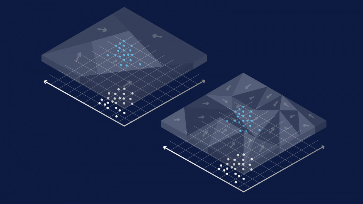
The goal of GAN training is to move some initial fake data distribution (produced by G) onto the real-data distribution until the discriminator or critic neural net can no longer tell the real and fake data apart. The problem is that G does not directly see the input data space; it only indirectly sees the space through a “mosaicglass” that is the gradient of D, i.e. ∇xD(x) (see the illustration below). If the “mosaic glass”,∇xD(x) always results in the same direction for different fake samples, then the starting cluster of fake samples cannot be dispersed onto different parts of the real-data distribution. In other words, for successful GAN training, it is not sufficient for D to perfectly classify the current real vs fake data points, but D needs to communicate to G how the different fake points are wrong in potentially different ways.
In the above illustration, semi-transparent mosaic glass represents the vector field ∇xD(x). Only the parts above the fake data points (white) pass transport information to G. When D models large input regions coarsely (left), G cannot move its mass accurately.
High diversity of learning signals for G = high diversity of activation patterns in D = concentration of D’s model capacity in the right place
Typically, D is a rectifier net. In the absence of the last sigmoid nonlinearity, D computes piecewise linear functions, meaning the learning signal to G is piecewise constant. The final sigmoid nonlinearity does not change the direction of the input gradient in each linear region, but merely shifts the scale of the gradient vectors. In other words, if two input data points activate the same set of neurons, the two inputs undergo the same linear transformation in the forward pass (modulo the final nonlinearity). Then, in the backward pass, they communicate the same gradient direction to G. Hence, the learning of G in GANs can be interpreted as the movement of the fake samples generated by G toward the real data distribution, guided by the (almost)piecewise constant vectorial signals according to input space partitioning by D.
Hence, the diversity and informativeness of learning signals to G are closely related to how D partitions the input space near fake data points, which in turn is directly manifested by the activation patterns in D on points from that region.
Here is an illustration of the ideas outlined so far in a synthetic 2D Mixture of Gaussian example:
The first column shows the data samples (blue) and generated samples (red) as they appear in data space. Each of the other columns demonstrates how the input data space gets partitioned according to the activation patterns at that layer, and the last column shows the probability of the images being real according to the output of D. Input points in a contiguous region of the same colour have the same activation pattern on that layer.
We can see that without BRE, G struggles to discover and lock onto the different modes, whereas with BRE, it quickly spreads its mass (even at iteration 1000, before 0:01 sec in the video). And later on, no matter how long we train the model, the samples do not escape from the found equilibrium.
Relationship to Arora’s work on model capacity and GAN
Arora and colleagues pointed out that in the case of final capacity neural nets, what GANs actually learn can be very different from the theoretical limit case where G and D have infinite capacity. In particular, a low capacity D cannot detect a lack of diversity (Corollary 3.2 of their paper). Our work states that even if D has enough potential capacity, it might not spread its capacity in a way that helps G learn how to generate diverse samples, and instead, we show a way to fix this problem.
How does it actually work? And how well does it work?
In practice, because of the connections among model capacity allocation, linear regions, and activation patterns, we can impact the first two items by working directly with activation patterns. The BRE regularizer encourages pairs of points in a mini-batch to have de-correlated activation patterns (or as much as possible while still performing the main discriminator/critic task). So, we take the activation pattern for one or more layers as a binary vectorial code for the corresponding input point and penalize the pairwise correlation. In practice, to make it differential and optimization-friendly, we soften the hard binarization with a scale-invariant soft-sign function (see Sec. 3.3 of the paper).
To reduce the number of hyperparameters introduced, we designed the BRE to be virtually unaffected by the difference in layer sizes. We achieved this by properly scaling with sizes and accounting for the effect of the Central Limit Theorem (see the relaxation by thresholding in Sec 3.3). In the end, there are only two design decisions/hyper-parameters: the weight of the BRE term, and the layers upon which it is applied. In practice, a weight of 1, coupled with application on all layers (barring the first and last layers that contain rectification) works reasonably well across all unsupervised problems.
Across a number of different architectures, BRE improves over both regular GANs as well as WGAN-GP. Even when the base architecture is already stable, like DCGAN, BRE can increase the speed of convergence. We also see improved semi-supervised learning classification accuracy on CIFAR10 and SVHN, when we take OpenAI’s feature matching code and add BRE.
Code available here.